algorithms of visual odometry and 3D terrain reconstruction
in planetary exploration.
The task of the PRoVisG Mars 3D challenge was to recon-
struct depth, camera trajectory and 3D maps of Mars land-
scapes observed by
MER
. The ExoMars PanCam test campaign
also focused on the 3D processing results, as they are an
essential component of mission planning and scientific data
analysis for the
ESA
’s ExoMars Rover mission, planned for
launch in 2020.
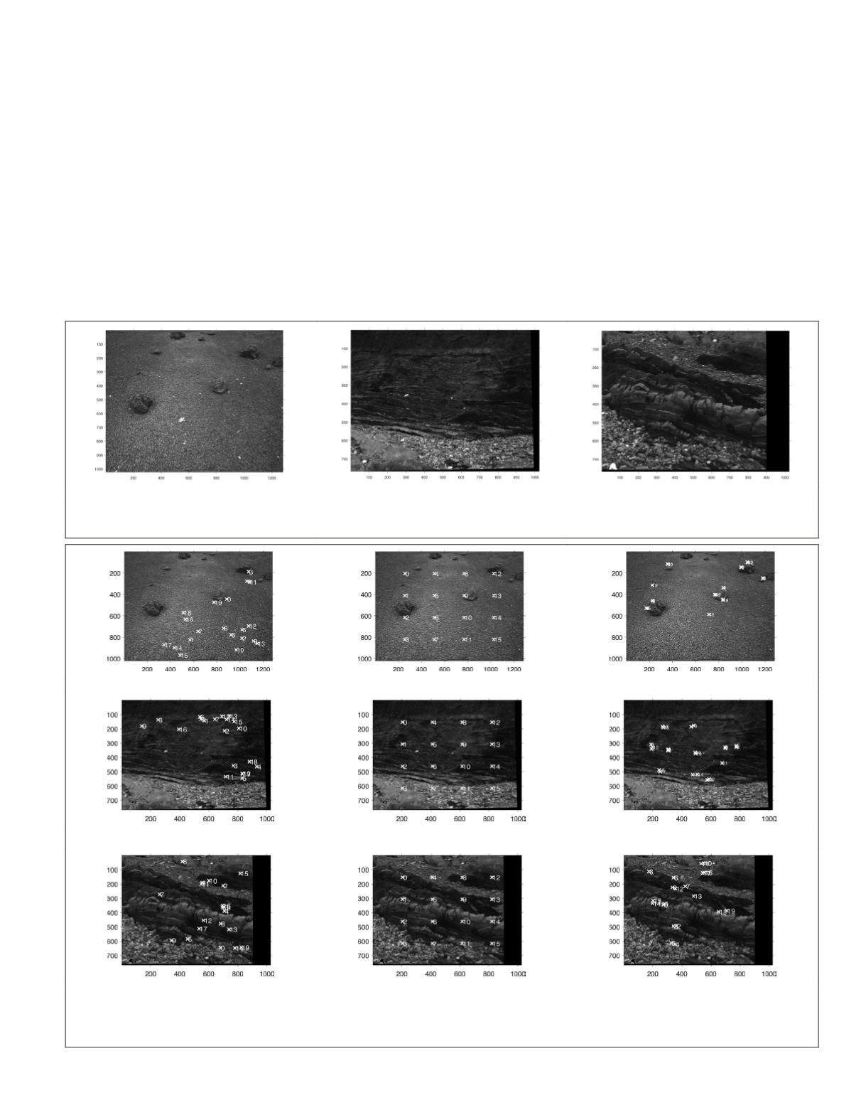
We demonstrate the evaluation with three test sequences,
taken from one of the PRoVisG Mars 3D challenge I datasets
(sets C33) and the ExoMars PanCam test campaign (“65246”
and “70000”). Examples of the images from each of these
three test sequences are shown in Figure 4. The evaluation
work demonstrated in this paper was achieved through a
workshop hosted at
UCL
-
MSSL
with 15 participants including
nine students and six trainers.
Test Datasets
During this stereo matching evaluation workshop, the stu-
dents were trained on how to use the StereoWS tool including
the stereo display, manual measurements, and a statistical
analysis procedure. In this workshop, we have collected man-
ual measurements, which were selected by different members
of the workshop.
During the manual measurement process, each participant
was asked to collect 20 feature based points, 16 regular grid
points, and 10 discontinuity tie-points for each pair of test
images shown in Figure 4. Figure 5 illustrates an example
of left tie-points of some of the test images (i.e., C33, 65246,
7000) prepared for measurement.
For the feature based tie-points (see the first column of
Figure 5), participants only needed to identify the corre-
sponding right points using the stereo display. Twenty left
points are selected from the extracted Scale Invariant Feature
(a)
(b)
(c)
Figure 4. Test datasets from
PRoVisG
Mars 3D Challenge and ExoMars PanCam Test Campaign, showing left-eye images
randomly picked from each test dataset: (a) C33, (b) 65246,and (c) 70000.
(a)
(b)
(c)
(d)
(e)
(f)
(g)
(h)
(i)
Figure 5. Example of left tie-points used in the stereo workshop: (a), (d), and (g) show 20 feature-based tie-points defined on
the test images shown in Figure 4(a), (b), and (c), respectively; (b), (e), and (h) show 16 regular grid tie-points for the same test
images; (c), (f), and (i) are for 20 tie-points around discontinuities.
PHOTOGRAMMETRIC ENGINEERING & REMOTE SENSING
March 2018
163


