WTLS
and the Procrustes algorithm (Mahboub, 2012; Fusiello,
A., and Crosilla, F., 2015).
Definition 2.
Given a set of the tie points defined in
F
r
and
denoted by (
T
1
,
T
2
, …,
T
n
), find the rigid translation
R
and rota-
tion
t
between the planetary rover’s body coordinate system
F
r
in varying stations.
Planetary Rover Pose Estimation in the
EIV
Mode
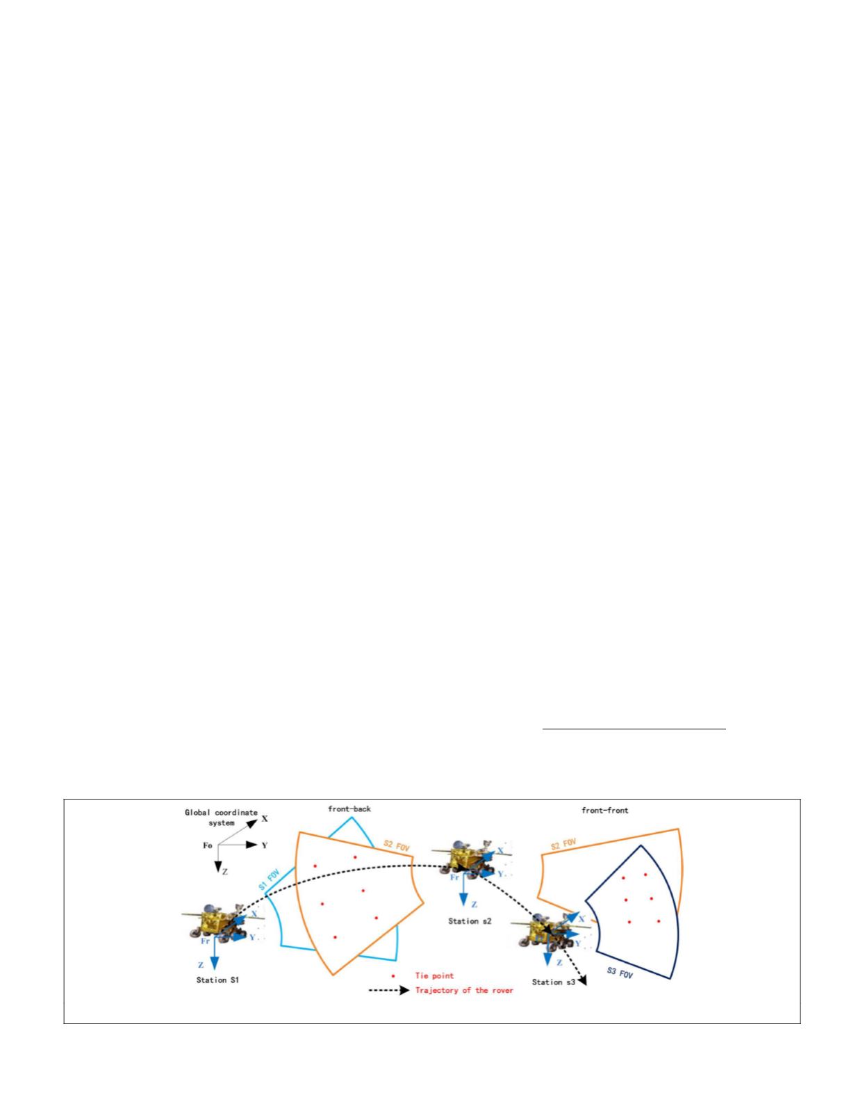
Figure 2 illustrates the planetary rover pose estimation for the
binocular camera system. Considering the image-capturing
model in the adjacent stations, there are two kinds of over-
lapping FOVs between binocular cameras denoted as “front-
back” and “front-front.” The “front” indicates that the images
are taken towards the front or side direction. Correspondingly,
the “back” indicates the back direction, which requires ob-
taining a sufficient number of tie points. As shown in Figure
2, there are some overlapping areas between the stereo
FOV
in
previous and current stations. For example, the overlapping
areas are in the front direction of the traverse in stations s1
and s3 but in the back direction in station s2.
As mentioned above, the new rover pose estimation
method can be described as:
B
=
ρ
C
ε
+
It
,
(15)
where
B
,
C
denotes the
n
×3 matrix containing all 3D coordinates of
the tie points (the coordinates of the former lie in the refer-
ence frame
F
r
in the previous station, and the latter lie in the
current station), and
n
is the number of the tie points,
ρ
is the scale change,
ε
denotes the 3×3 rotation matrix containing three indepen-
dent parameters named pitch angle
ω
, roll angle
φ
and yaw
angle
κ
,
t
denotes the 1×3 translation vector, with
t
= (
Δ
X
,
Δ
Y
,
Δ
Z
),
and
I
denotes the identity vector.
In view of the random errors in matrixes
B
and
C
, Equation
15) should be further extended to the
EIV
model:
B
+
E
B
=
ρ
(
C
+
E
C
)
ε
+
It
,
(16)
( )
e
E
e
E
Q
Q
B
B
C
C
B
C
=
=
( )
vec
vec
N
~
,
0
0
0
0
0
2
σ
where
E
B
,
E
C
denotes the
n
×3 matrix of added random errors in coef-
ficient matrix
B
and coefficient matrix
C
, and
Q
B
,
Q
C
denotes
the 3
n
×3
n
symmetric positive-definite cofactor
matrix.
Similar to the relative orientation method in previously dis-
cussed, the coefficient matrix is complicated when we adopt
the
OLS
solution of Equation 15. In addition, the dependency
on the initial value of the pitch angle
ω
, roll angle
φ
and yaw
angle
κ
of the rover should be considered. In the various
solutions of the 3D similarity transformation model, the Pro-
crustes algorithmhas the characteristics of steady arithmetic,
high precision, and non-iterative calculation, thus offering a
profitable reference for the visual localization of the rover. In
other words, the Procrustes algorithm can avoid pitfalls in the
OLS
solution.
In (Mahboub, 2012), the author proposes that the rotation
matrix based on
OLS
equals the solution on
EIV
when import-
ing the Procrustes algorithm:
ε
=
UV
T
,
(17)
where
U
,
V
denotes the left and right singular matrixes of
C
–
T
T
– by
singular value decomposition,
B
– =
W
n
τ
B
denotes the normalized matrix,
C
– =
W
n
τ
C
denotes the normalized matrix,
W
n
denotes the
n
×
n
positive-definite weight diagonal matrix,
which will be described in the next Section, and
τ
=
I
– (
I
T
W
n
W
n
I
)
–1
(
II
T
W
n
W
n
) is the idempotent matrix.
In (Mahboub and Sharifi, 2013), the translation vector
τ
is
simply given as
τ
= (
I
T
W
n
W
n
I
)
–1
I
T
W
n
W
n
(
B
–
ρ
C
ε
).
(18)
Set
C
′
=
C
ε
; we can then calculate the scale change
ρ
from
(Fang, 2013):
tr(
B
T
C
′
)
ρ
2
+ tr(
C
T
C
–
B
T
B
)
ρ
– tr(
B
T
C
′
) =
0
.
(19)
The estimated value of the unknown variance component
σ
2
0
, regardless of the translation vector
τ
and the scale change
ρ
, can be represented as:
(
)
I
B
(
)
B C
σ
ε
ε ε
ε
0
2
3 3
3 7
=
−
+
−
(
)
(
)
−
×
tr
n
C
T
T
.
(20)
Figure 2. Illustration of planetary rover pose estimation
PHOTOGRAMMETRIC ENGINEERING & REMOTE SENSING
October 2018
609


