is introduced based on the image space compensated param-
eters
Δ
c
and
Δ
r
, which is expressed as:
c c
Num H
Den
H
c c
r r
Num H
s
s n n n
s n n n
s
L n n n
= ⋅
+
= ⋅
( , ,
)
( , ,
)
( , ,
)
φ λ
φ λ
φ λ
+
0
∆
Den
H
r
r
L n n n
( , ,
)
φ λ
+ +
0
∆
(7)
The laser data can then be viewed as a control point with
accuracy elevation for combined adjustment (Li
et al
., 2016a).
Thus, the contribution of this paper is a discussion of the dis-
tribution of the
ZY3-02
SLA
points and the mapping result after
integration without
GCPs
for
ZY3-02
satellite optical images,
which represents the combination of the laser altimetry data
and stereo images from the same satellite for Earth observa-
tion.
Adjustment with RSM and Ranging Constraint (RSM_RC)
The rigorous sensor model of
HRSI
can be described as follows
(Tang
et al
., 2015):
X
Y
Z
X
Y
Z
mR R R
G
G
G
J
WGS
star
J
body
=
+
2000
84 2000
star
camera
body
y
x
R
tan( )
tan( )
ψ
ψ
−
1
(8)
where (
ψ
x
,
ψ
y
) are the look angles of the detector on the
charged coupled device (
CCD
) linear array, (
X, Y, Z
) are the
three-dimensional coordinates of the object point correspond-
ing to the image point, and (
X
G
, Y
G
, Z
G
) are the positions of
the camera imaging center in the
WGS84
coordinate system.
R
camera
body
refers to the installation matrix of the camera,
R
body
star
represents the rotation relationship from the satellite body to
the star tracker,
R
star
J
2000
refers to the attitude determination
reference coordinate system to the J2000 coordinate system at
imaging time,
R
J
WGS
2000
84
refers to the rotation matrix from the
J2000 coordinate to the
WGS84
geocentric coordinate system at
imaging time and
m
is the scale factor.
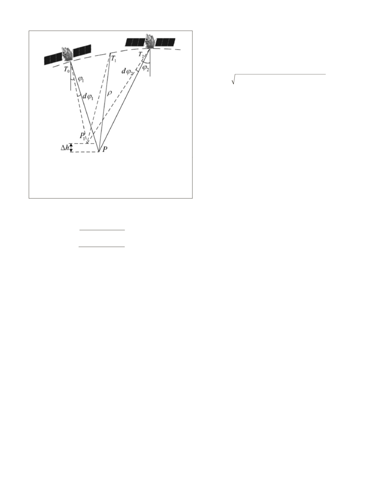
A laser altimeter and stereo camera on the same satellite
platform is illustrated in Figure 6. The stereo images are ob-
tained at times
T
0
and
T
2
. The laser ranging value is obtained
at time
T
1
, and
P
and
P
1
are the corresponding points between
the laser and stereo images.
The laser ranging constraint formula can be expressed as:
F X X Y Y Z Z
p S
p S
p S
=
− + − + − − =
(
) (
) (
)
2
2
2
0
ρ
(9)
where (
X
s
, Y
s
, Z
s
) are the positions of the laser reference point
on the satellite in the
WGS84
coordinate system, (
X
p
, Y
p
, Z
p
) are
the object space coordinates of the laser footprint point in the
WGS84
coordinate system, and
ρ
is the precise laser ranging
value after atmospheric and systematic error corrections.
The attitude-compensated model can be expressed as
Equations 10 and 11.
= +
= +
= +
φ φ φ
ω ω ω
κ κ κ
t
t
t
∆
∆
∆
0
0
0
(10)
∆ = + + − + − +
∆ = + + − + − +
φ φ
ω ω
0 0 1 0 2 0
2
0 0 1 0 2 0
2
a a t t
a t t
b b t t
b t t
(
)
(
)
(
)
(
)
∆ = + + − + − +
κ κ
0 0 1 0 2 0
2
c c t t
c t t
(
)
(
)
(11)
where, (
φ
0
,
ω
0
,
κ
0
) and (
Δ
φ
,
Δ
ω
,
Δ
κ
) are the attitude-measured
and -compensated value, respectively.
a
i
, b
i
, c
i
(
i
= 0,1,2, … )
are the compensated coefficients,
t
is the imaging time, and
t
0
is the time of the reference attitude-measured value. In this
paper, we use only the offset parameters and one-polynomial
coefficient, respectively.
The combined adjustment laser altimetry data and stereo
images from Equations 9, 10, and 11 can then be implemented
to compensate the satellite attitude, especially the angle
φ
, with
the laser ranging constraint. And the resolved method of the ad-
justment formulas is equal to Li
et al
.(2016a). Then, the eleva-
tion accuracy of stereo images can be improved without
GCPs
.
Experiment and Results
Experiment
Combined Adjustment of Laser Altimetry Data and Stereo Images
In the four experimental regions, the
ZY3-02
SLA
points are se-
lected as elevation control data, and the combined adjustment
with
RPCs
and compensated model is implemented. The result
of combined adjustment with
RFM
or RSM is compared in the
first and second experimental regions, where the laser data
and stereo images are collected synchronously from the same
orbit. The distribution of different types of points is depicted
in Figure 7. We tried to use different types of points, which
are described in Table 4. The elevation control points (ab-
breviated as V) are derived from the
ZY3-02
SLA
or
GLAS
data,
and the selecting strategy is described in the Materials and
Methods Section, which contains the terrain and the image
registration result. The horizontal control points (abbreviated
as H) are selected from the checkpoints; when used as the
horizontal control, the checkpoints need to be subtracted.
Distribution of Laser Control Data
In the experiment, we also tested the impact of laser elevation
control point distribution on adjustment accuracy. Figure 8
shows a total of six different distribution of laser elevation
control points implemented in the first experimental region.
Figure 6. Illustration of laser ranging constraint and stereo
images derived from the same satellite.
P
is true point on
the ground, and the laser ranging value is
ρ
; the measured
attitude angles along the track of the stereo images is
φ
1
and
φ
2
, and the errors are
d
φ
1
and
d
φ
2
, respectively. Elevation
deviation between
P
and
P
1
is
Δ
h
.
PHOTOGRAMMETRIC ENGINEERING & REMOTE SENSING
September 2018
573


