large-area or global mapping, especially in the planetary map-
ping field (Gwinner
et al.
2010, 2016; Preusker
et al.
2017).
Mapping with partitions is an engineering method for parallel
processing and dealing with huge amounts of data. It is also a
feasible way to improve the processing precision when the data
are of different quality in different regions, which is very com-
mon with the planetary orbital images (Gwinner
et al.
2016).
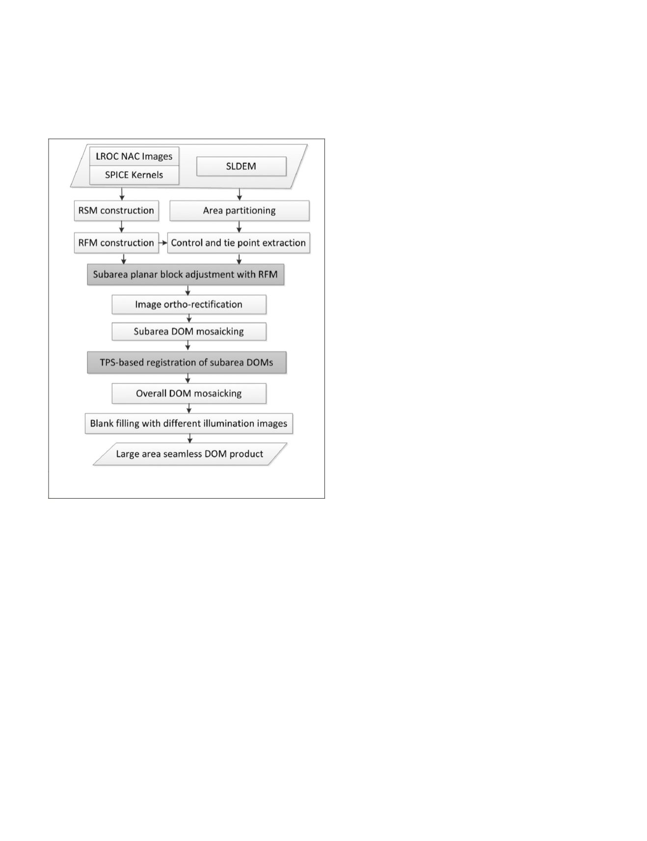
Figure 2. Flowchart of large-area high-reso
DOM
generation.
A planar block adjustment with control points was used
in each subarea to ensure the relative consistency among the
LROC NAC
images and the absolute accuracy to the control
source. The rational function model (
RFM
) of the image was
refined during the block adjustment. Via the block adjust-
ment, geometric inconsistencies between adjacent
LROC NAC
images within each subarea can be effectively reduced. Subse-
quently, the
DOM
of each image was automatically generated,
and the
DOMs
within each subarea were mosaicked together.
Because of the resolution limitation of the reference source,
some positional inconsistencies between the
DOM
mosaics of
neighboring subareas remained. Therefore, a
TPS
model–based
image registration was applied to the generated subarea
DOM
mosaics. To maintain the grayscale and contrast homogeneity,
a histogram matching–based grayscale balancing method was
applied to all the
DOMs
. Finally, a seamless
DOM
product of the
entire planned landing area was generated via mosaicking.
It is worth mentioning that the contrast of the
WAC
mosaic
is lower than most
NAC
images, which causes the
NAC
mo-
saic to appear a little grayish. Nevertheless, the
WAC
mosaic
provides a very consistent source in a larger scale so that the
produced mosaic has a good radiometric consistency, which
can satisfy most of the applications at present. Color balanc-
ing for large-area mapping deserves future research.
Geometric Models of Orbital Imagery
The geometric model of the imagery is the mathematical basis
for block adjustment as well as the image ortho-rectification.
It builds the relationship between object-space coordinates
and image-space coordinates.
The rigorous sensor model (
RSM
) of an image represents the
imaging process by collinearity equations with interior ori-
entation (
IO
) parameters and exterior orientation (
EO
) param-
eters (Di
et al.
2014; Henriksen
et al.
2016; Liu
et al.
2017).
The generic geometric model of an image fits the relationship
between the image and ground coordinates via mathematical
functions, the parameters of which have no physical mean-
ing related to the imaging process. The most commonly used
generic geometric model is the
RFM
. The
RFM
has the advan-
tages of high fitting precision, simple and uniform form, high
calculation speed, and imaging sensor independence. It has
already been widely accepted that the
RFM
can approximate
the
RSM
at a precision of 1/100 pixel in image space (Liu
et al.
2016, 2017) such that it can be used to replace
RSM
without a
loss of accuracy.
The
RSM
of the
NAC
imagery was constructed using the
IO
and
EO
parameters recorded in
SPICE
kernels (NAIF 2014). It
can be generally described (Di
et al.
2014) as
X X
Y Y
Z Z
R R R
x
y
f
R
x
y
f
s
s
s
ol bo ib
−
−
−
=
−
=
−
λ
λ
(1)
where (
x
,
y
) are the focal plane image coordinates;
f
is the
focal length; (
X
,
Y
,
Z
) and (
X
s
,
Y
s
,
Z
s
) represent the lunar-
surface-point coordinates and the position of optical center in
the lunar body-fixed coordinate system (LBF), respectively;
λ
is a scale factor;
R
ib
is the rotational matrix from the image
space coordinate system to the spacecraft body coordinate
system (BCS);
R
bo
is the rotational matrix from the BCS to
the orbit coordinate system (OCS);
R
ol
is the rotational matrix
from the OCS to the LBF; and
R
is the combination of these
atrices and can be constructed using the three
eters (
ω
,
φ
,
κ
) (Liu
et al.
2017).
for linear array push-broom images, each line
et of
EO
parameters. Because the time interval
of the orbit measurement is much longer than that of the line
scanning, only a small portion of the image lines have
EO
pa-
rameters from direct measurements. To obtain the
EO
param-
eters of all image lines via interpolation, the
EO
parameters
are usually interpolated with respect to the scan time
t
(Di
et
al.
2014). There are many methods for
EO
parameter interpola-
tion. The polynomial representation is a feasible choice and
widely used. The third-order polynomial is chosen to model
the
EO
parameters as shown in Equation 2:
X t a a t a t a t
s
( )
= + + +
0 1 2
2
3
3
Y t b b t b t b t
s
( )
= + + +
0 1 2
2
3
3
Z t c c t c t c t
s
( )
= + + +
0 1 2
2
3
3
(2)
φ
( )
t d d t d t d t
= + + +
0 1 2
2
3
3
ω
( )
t e e t e t e t
= + + +
0 1 2
2
3
3
κ
( )
t f f t f t f t
= + + +
0 1 2
2
3
3
where
a
0
,
a
1
, …,
f
3
are the polynomial coefficients of the six
EO
parameters (
X
s
,
Y
s
,
Z
s
,
ω
,
φ
,
κ
).
The focal plane image coordinates (
x
,
y
) can be obtained by
transforming from the image coordinates (
row
,
sample
) using
IO
parameters as follows:
PHOTOGRAMMETRIC ENGINEERING & REMOTE SENSING
July 2019
483


