where (
d
i
a
,
d
i
p
,
d
i
n
) 1
≤
i
≤
N
is the triplet constructed using the
sampling rule in the section “Sampling Strategy”;
λ
is the
L
2
regularization factor, also known as weight decay; and
Θ
is the
vector of learned parameters for the network. We should note
that the difference of Equation 10 from former loss functions is
the inclusion of 1 in the logarithm, which changes the behav-
ior of the loss to a logistic one. Without the loss of generality,
to simplify the discussion, let
x
2
= dist(
d
i
a
,
d
i
p
) – dist(
d
i
a
,
d
i
n
).
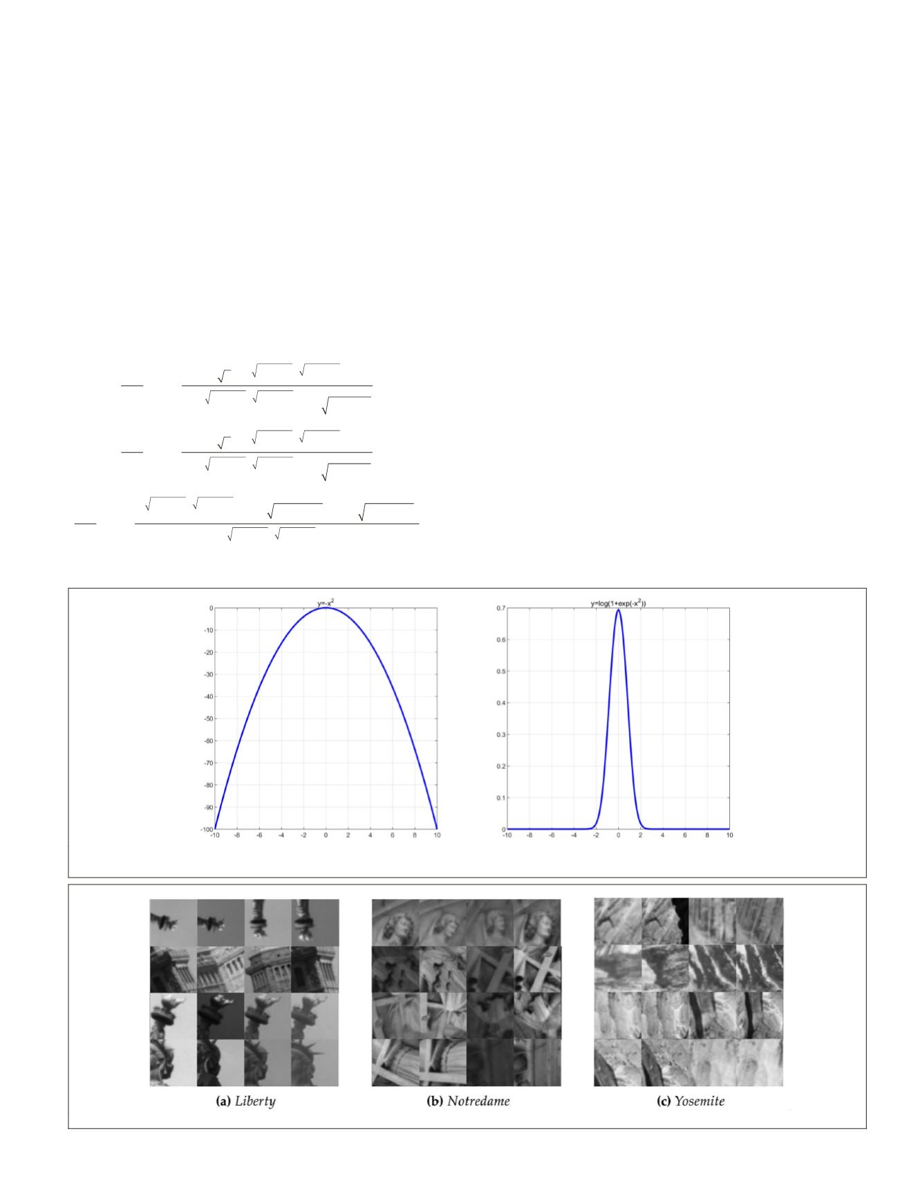
Using this scheme, our proposed function can be considered
as
y
= log(1 +
e
–x
2
), while the common loss function is
y
= –
x
2
.
Plotting both functions, one can see from the plot on the right
in Figure 3 that the proposed function has well-defined upper
and lower bounds, eliminating the requirement for setting
margins. In contrast, the commonly used loss on the left re-
quires setting margins. Additionally, the proposed logistic loss
has faster convergence properties due to the slope of the tan-
gent in back-propagation which is computed from the gradient
of the loss
L
with respect to
d
i
a
,
d
i
p
, and
d
i
n
:
−
−
∂
∂
= ∑
−
=
−
(
−
− −
(
L
d
d e
e
p
i
N
a
d d
d d
d d
n
a p
a p
a
1
2 2
2 2
2 2
2
2
∂
∂
= ∑
−
=
−
− −
(
)
−
− −
2
2
1
2 2
2 2
2 2
2 2
L
d
d e
e
n
i
N
a
d d
d d
n
d d
d d
a p
a
a p
a n
a p
n
i
N
d d
d d
n
n
a
d d
L
d
e
d
d d
n
a p
a
(
)
=
−
− −
(
)
+
−
∂
∂
= ∑
1 1
2 2
1
2 2
2 2
/
d
d d
e
p
a p
d d
d d
n
a p
a
/
2 2
1
2 2
2 2
−
(
)
+
−
− −
(
)
(11)
Implementation Details
We used the PyTorch library (Paszke
et al.
2017) to train the
proposed network. All the image patches are resized to 32×32
pixels. The optimization algorithm chosen is the stochas-
tic gradient descent algorithm with a learning rate of 10, a
momentum of 0.9, and an L2 regularization factor of 0.00001.
There are 1024 triplet samples in a batch, and the network
was trained 30 epochs for every training data set. Following
Mishchuk
et al.
(2017), data augmentation, including random
flipping and rotating 90 degrees for three image patches in a
triplet sample, was applied.
Experiments and Analysis
In this section, we evaluate the effectiveness of the proposed de-
scriptor on two publicly available patch evaluation benchmark
data sets and two real remote sensing images. We first introduce
the data sets and then present the experimental results in detail.
n
et al.
2011), also known as the
enchmark data set widely used for
descriptor to distinguish match-
ing image pairs from nonmatching image pairs. There are
three image sets—Liberty, Notredame, and Yosemite—in the
data set, each of which contains more than 450K local image
patches with a resolution of 64×64 pixels. The patches, gener-
ated from real-world images, are extracted using a difference
of Gaussians detector and verified through the 3D model.
Thus, all the matching patches are from the same 3D physical
point. Although the detector has already normalized the scale
and orientation of the patch, the images in the data set still
have variations in view and illumination changes. Figure 4
shows some examples from the data set.
Figure 3. (Left) The commonly explored loss function with no margins. (Right) The proposed logistic loss function with
implicitly well-defined margins.
Figure 4. Some examples of the matching image pairs in three sets of the Brown data set.
PHOTOGRAMMETRIC ENGINEERING & REMOTE SENSING
September 2019
677


