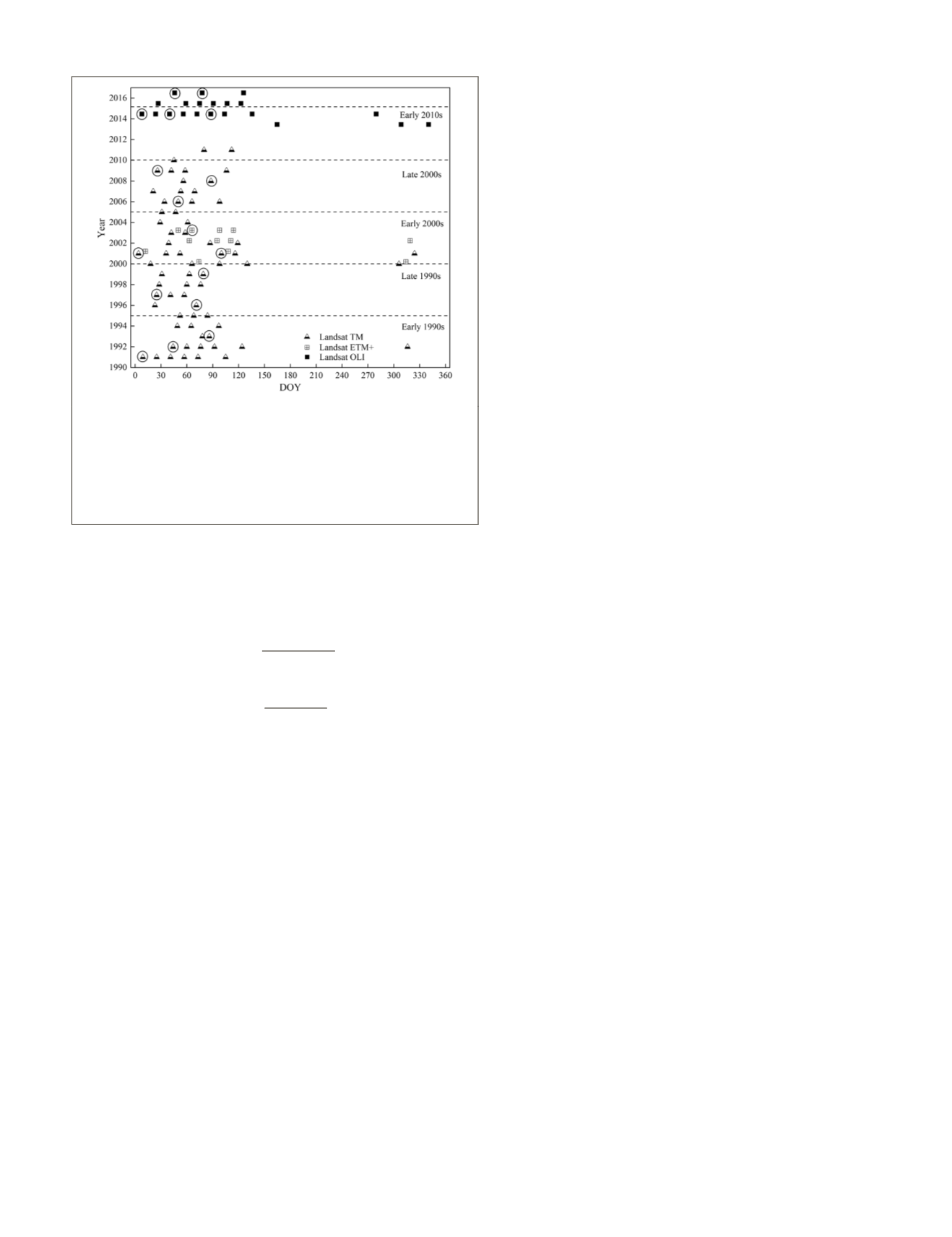
periods: the early 1990s (1991–1995), late 1990s (1996–2000),
early 2000s (2001–2005), late 2000s (2006–2010), and early
2010s (2011–2015). We also used the Landsat-derived
NDVI
as auxiliary mask data for mapping deciduous rubber planta-
tions (pixels). The formulae used in this study are
NBR
NIR SWIR2
NIR SWIR2
=
−
+
ρ ρ
ρ ρ
(1)
NDVI
NIR Red
NIR Red
=
−
+
ρ ρ
ρ ρ
,
(2)
where
ρ
Red
,
ρ
NIR
, and
ρ
SWIR2
denote the values of surface reflec-
tance for the red (Band 3),
NIR
(Band 4), and
SWRI
2 (Band 7)
bands in
TM
/
ETM+
sensors, and the red (Band 4),
NIR
(Band 5),
and SWRI 2 bands (Band 7) in
OLI
sensor.
Field-Survey Data
The ground-reference data used in this study comprise field
GPS
points,
GPS
trip routes, and geo-tagged photos that were
collected in two field surveys, as well as very high-resolution
Google Earth (
GE
) imagery. One survey was carried out in
the Lancang-Mekong River Basin between late February and
mid-March 2013. Hybrid
GPS
cameras (Casio Exilim
EX-H20G
)
and handheld
GPS
receivers (Trimble 3B) were used to capture
497 geo-referenced landscape photos and 253
GPS
points to
understand the differences in land use types within Xish-
uangbanna (Figure 1a). The other was carried out within the
border region of Yunnan Province in early February 2015. A
Casio Exilim
EX-H20G
camera and a Trimble 3B
GPS
receiver
were used to collect more than 1000 geo-tagged photos
within Xishuangbanna (Figure 1a). Our field-survey sampling
strategy emphasized deciduous rubber plantations and other
land use types, such as natural forests, swidden agriculture,
and croplands (e.g., paddy rice). Photos were used to record
specific geographical information (e.g., latitude, longitude,
altitude, and lens direction) of various land use types and
then transformed into a shape-file format using Google Picasa
software (Version 3).
Meanwhile, we also conducted visual cross-comparisons
of landscape differences between recently acquired
OLI
(2015
and 2016) and
GE
images with local land cover types in
situ during the field trips, by means of a vehicle-based
GPS
receiver (
HOLUX M-215+
) via
ArcGIS
platform. Our geo-tagged
photos were used for two purposes. One was to define points
of interest (
POIs
) for studying the temporal variations in
NDVI
and
NBR
between deciduous rubber plantations and natural
evergreen forests at the pixel scale during different phases.
We therefore selected 18 training sites that comprised largely
homogeneous patches of deciduous rubber plantations (12
POIs
) and natural evergreen forests (six
POIs
; Figure 1b). In all
cases, the vertical distance of any
POI
to the field route was
less than 2.0 km, while the linear distance between any two
adjacent sites ranged between 0.83 and 11.6 km (an average of
7.3 km). The other purpose was to generate regions of interest
(
ROIs
) and establish
NBR
temporal profiles of deciduous rubber
plantations. Training
ROIs
for deciduous rubber plantations
itized using both geo-tagged photos
l set of 38
ROIs
and a total of 1548
POIs
and
ROIs
were uncontaminated
Landsat-Based Phenology Analysis of Deciduous Rubber Plantations
Over the course of two field surveys, we noticed that decidu-
ous rubber plantations within the study area undergo obvious
landscape changes as their leaves turn yellow, defoliate, and
emerge, and the canopy recovers (e.g., Ph1 and Ph2 in Figure
3). We further used a set of 70 quasi-annual partial Landsat
images to illustrate phenological differences of deciduous
rubber plantations in false-color composite maps (i.e., R/G/B
= Bands 5/4/3 in
TM
and
ETM+
, 6/5/4 in
OLI
) between 1991 and
2016 (Figure 3).
The imaging features shown in Figure 3 (especially in
color) highlight the fact that deciduous rubber plantations
differ greatly from natural evergreen forests during defolia-
tion and foliation phases. In Figure 3, the pixels of deciduous
rubber plantations are purple during the defoliation phase as
their leaves’ moisture content decreases, while those of natu-
ral evergreen forests remain light green. Similarly, deciduous
rubber plantations are characterized by bright green patches
during the foliation phase, while those of natural evergreen
forests are dark green. These differences mean that the pixels
of deciduous rubber plantations are easily visually distin-
guished during defoliation and foliation phases.
Assessing the timing and variations of biological rhythms
is important for developing robust algorithms for mapping
deciduous rubber plantations. Figure 4 shows the temporal
dynamics of
NBR
of deciduous rubber plantations and natu-
ral evergreen forests for the five historical epochs—the early
1990s (Figure 4a), late 1990s (Figure 4b), early 2000s (Figure
4c), late 2000s (Figure 4d), and early 2010s (Figure 4e). The
temporal development of average
NBR
values of deciduous
rubber plantations conforms to a quasi-U-shaped distribution
(ranging between 0.15 and 0.65) during the dry season, while
those of natural evergreen forests remain persistently stable
(nearly 0.70). Figure 4f shows that the mean
NBR
values for
deciduous rubber plantations remained closely equal to those
of natural evergreen forests during the foliation phase within
each epoch, while their differences were much more signifi-
cant during the defoliation phase.
Figure 5 gives a further seasonal dynamics of
NBR
derived
from
LTS
imagery for the early 1990s (Figure 5a), late 1990s
(Figure 5b), early 2000s (Figure 5c), late 2000s (Figure 5d),
and early 2010s (Figure 5e). The gray rectangles in Figure
5 clearly show the rapid phenological transition of decidu-
ous rubber plantations, especially between February and
April. It is also clear that the
NBR
values of deciduous rubber
Figure 2. Acquisition dates (i.e., da
Landsat Thematic Mapper (
TM
), Enhanced
TM
Plus (
ETM+
),
and Operational Land Imager (
OLI
) images with cloud cover
≥
30% used for construction of the Normalized Burn Ratio
(
NBR
) in Xishuangbanna. The Landsat Time Series (
LTS
)
scenes labeled in the black circle were used to generate
maps of deciduous rubber plantations.
PHOTOGRAMMETRIC ENGINEERING & REMOTE SENSING
September 2019
689


