with heavy cloud cover, cloud-free parts of the image can be
used to enhance the temporal sampling frequency. A signifi-
cant number of high quality pixels in the Landsat
SLC
-off
ETM
imagery are also useful for time series data analysis. Therefore,
all available Landsat 5, 7, and 8
ARD
imagery were obtained to
develop a dense time series stack. We also downloaded two
recent
NLCD
map products (
NLCD
2001 and
NLCD
2011) from
the Multi-Resolution Land Characteristics Consortium (http://
). Overall accuracies for
NLCD
are approximate-
ly 85% and individual class accuracies ranged from 79% to
91% for Anderson Level I classes (Wickham
et al.
2010).
Data Preprocessing
We derived
NDVI
for each Landsat image from 1988 to 2017
and stacked all
NDVI
layers to develop a
NDVI
time series stack.
No additional data preprocessing steps were needed before
NDVI
calculation because Landsat
ARD
surface reflectance data
come readily processed to the highest scientific standards.
The main reason to use
NDVI
time series for our annual urban
mapping was to reduce data dimensionality—one
NDVI
layer
versus six surface reflectance bands. In addition,
NDVI
is
good indicator of vegetation condition and status; new urban
development typically involves vegetation clear-cut and
NDVI
change (Lunetta
et al.
2006, Shao
et al.
2011).
To reduce cloud contamination, we applied an
MVC
algorithm to the original
NDVI
time series to derive monthly
NDVI
layers. Each monthly
NDVI
layer is a composite image
representing the highest observed
NDVI
value for each pixel
in a given compositing month. The
same
MVC
algorithm (Holben 1986)
was used as the compositing algo-
rithm in developing 16-day
MODIS
NDVI
products (Huete
et al.
2002);
here, we applied it to 30 m Land-
sat time series. The monthly
NDVI
images appeared to be noisy, with a
significant amount of missing data
due to image availability and cloud
impacts. Thus, to further reduce
cloud impacts and data volume, we
applied the
MVC
algorithm to the
NDVI
time series to derive annual
NDVI
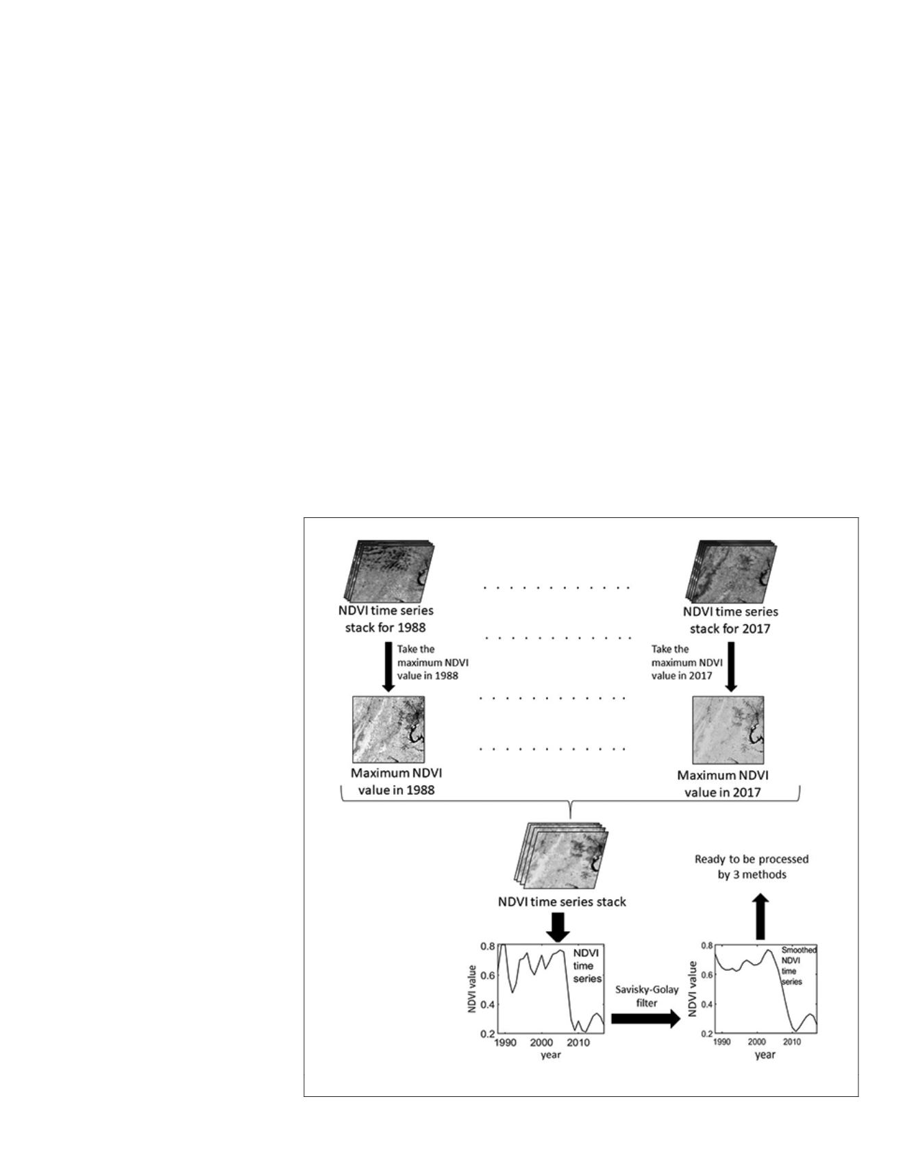
layer from 1988 to 2017. The
resultant annual
NDVI
layers were
stacked to construct annual
NDVI
time series—each pixel has 30
NDVI
values covering years from 1988 to
2017. We applied a Savitzky-Golay
smoothing algorithm to remove
pseudo hikes and drops from
the annual
NDVI
time-series. The
Savitzky-Golay filter is among the
best performers with respect to ease
of implementation and robustness
of results (Chen
et al.
2004; Jia
et
al.
2014; Shao
et al.
2016). Figure 2
shows the flowchart for the above-
described data processing steps.
Annual Urban Mapping
We used
NLCD
as our primary refer-
ence data to evaluate our annual
urban mapping methods. Start-
ing with
NLCD
2001, each release
of
NLCD
divides urban areas into
four classes: (a) developed open
space (< 20% impervious cover;
class code 21), (b) low-intensity
developed (20–49% impervious cover; class code 22), (c) me-
dium-intensity developed (50–79% impervious cover; class
code 23), and (d) high-intensity developed (
≥
80% impervi-
ous cover; class code 24) (Homer
et al.
2015). By comparing
to higher resolution urban map, Irwin and Bockstael (2007)
stated that
NLCD
has relatively low classification accuracy for
open space and low intensity urban classes, mainly due to
limitations of 30 m Landsat resolution. Therefore, it is more
realistic to focus on medium-high intensity urban pixels
(
NLCD
classes 23 and 24) for better mapping accuracy. Using
2001
NLCD
and 2011
NLCD
as reference, we identified all pixels
influenced by urbanization processes (from nonurban land
cover to medium-high intensity urban) and pixels influenced
by urban intensification processes (from open space/low
intensity urban to medium-high intensity urban) during the
10-year time period. These
NLCD
-derived urban change pixels
were principal targets for further detection of their corre-
sponding urban change years.
In the following section, we describe three time series analy-
ses used for identifying the specific year of urban change. For
each time series change detection method, we examined input
data for two time series, 1998–2014 and 1988–2017, to evaluate
how length of input
NDVI
time series affect mapping accuracy.
Minimum-Value Method
For the minimum-value method, our assumption was that
the minimum
NDVI
value within each
NDVI
time series should
match well with specific urban change year. It is expected to see
a significant decrease of the
NDVI
value if a forest/agricultural
Figure 2. Flowchart of data preprocessing.
PHOTOGRAMMETRIC ENGINEERING & REMOTE SENSING
October 2019
717


