The proposed algorithm needs to use the
LMB-CNN
to ex-
tract the deep features, which are the output from the first full
connection layer. The feature dimension is set to 256 in this
article, as shown in Figure 2. To train the network, we treat it
as a two-class classification task and end the
LMB-CNN
with a
softmax function. The selected loss function is cross-entropy
loss, which is described in Equation 3:
(
)
J
m
y
h x
y
h x
i
i
i
m
i
i
( )
log
log
.
( )
( )
( )
( )
θ
θ
θ
= −
(
)
+ −
(
)
−
(
)
(
)
=
∑
1
1
1
1
(3)
For optimization, we apply the Adam algorithms described
in Kingma and Ba (2014), the initial learning rate is set to
0.0003, and the batch size is set to 64. The total number of
iterations is 200 000. The network is implemented by Keras,
and all other parameters are default values.
The training process is illustrated in Figure 3, which
shows that the networks converge rapidly and stably. The
speed and accuracy of
LMB-CNN
will be demonstrated in the
experiment section.
Segment Feature Maps by FCN
The above steps extracted the deep features of each block, and
the feature dimension was 256. Based on the spatial position
of image blocks, the deep features were rearranged into 256
channel feature maps, similar to the output of a series of con-
volutional layers. The first nine feature maps of the sample
image are shown in Figure 4.
In the second step of the proposed method, the recon-
structed feature maps are treated as the input of an
FCN
model. Considering the calculation speed, the basic structure
of
LMB-CNN
is reused by
FCN
. However, the pooling operations
and the full connection layers are removed to keep the feature
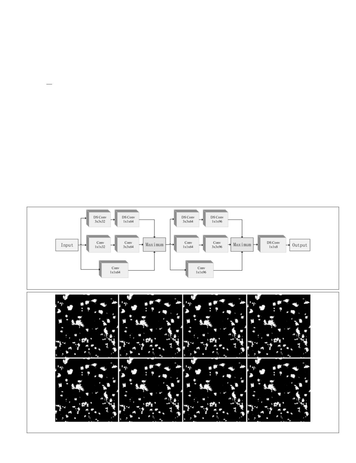
map’s size unchanged. The structure of the
FCN
model is
shown in Figure 5, taking an eight-kernel depthwise separable
convolutional layer activated by a sigmoid function as the end
of the network, which outputs eight channel segmentation
masks to improve the segmentation reliability. Intuitively,
voting on the multiple decisions is better than only one deci-
sion since different output channels consider different inner
characteristics of the input features. Figure 6 gives an intui-
tive view of the eight outputs. Experimental results in Table 4
show that the voting strategy can reduce the false alarms and
missing alarms.
Because our problem is binary classification, it is conve-
nient to measure the difference between the output results
of each channel and groundtruth by the mean square error. It
also avoids the probability calculation when using cross en-
tropy. In addition, for our problem, the false alarms and miss-
ing alarm we are concerned about are usually located on the
boundary of the built-up area. The sigmoid output probabili-
ties of these samples are usually around 0.5 if we use cross
entropy. However, the mean square error can highlight the
contributions of these samples. Therefore, the loss function
based on the square error is adopted for training the
FCN
mod-
el, but the output is divided into three parts when calculating
Figure 5. The structure of the
FCN
mo
Figure 6. The eight preliminary segmentation masks that are produced by the
FCN
model.
PHOTOGRAMMETRIC ENGINEERING & REMOTE SENSING
October 2019
741


