the loss function: correct classification, false alarm, and miss-
ing alarm. The specific loss function is as follows:
=
+
∑
∑
L
h x y
h x y
i
i
y
i
i
y
p
p
i
i
i
i
( )
( )
( )
,
θ
α
θ
θ
( )
−
( )
−
( )
( )
( )
( )
=
= =
( )
( )
2
1 0
2
0 1
2
+
( )
−
( )
( )
= =
( )
∑
β
θ
h x y
i
i
y p
i
i
( )
,
,
(4)
where
h
θ
(
x
(
i
)
) indicates the output of the
FCN
model and
y
(
i
)
is
the ground truth,
y
(
i
)
= 1 represents the built-up area,
y
(
i
)
= 0
is the non–built-up area,
α
and
β
are the parameters that can
be specified, and
p
(
i
)
is the threshold discriminant result of
h
θ
(
x
(
i
)
), which is formulized as follows:
p
h x
h x
i
i
i
( )
,
.
.
,
.
=
( )
≤
( )
>
( )
( )
0
0 5
1
0 5
θ
θ
(5)
By adjusting the weights of the loss function, the contribu-
tion of the error classification part can be increased to avoid
being covered by the correct classification part. In fact, after
a certain number of iterations, more than 90% of the units
will be classified correctly. The optimization process is the
same as
LMB-CNN
, except that the initial learning rate is set to
0.0001. The data set will be described in the next section.
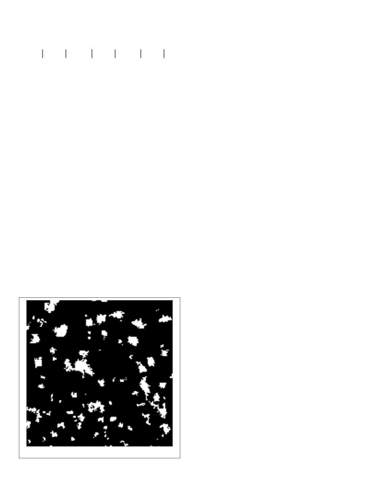
Voting on the Preliminary Segmentation Results
The eight segmentation masks of the
FCN
model are shown
in Figure 6. There is an approximate 6% difference between
each pair of masks, which indicates that each block may have
varied binary values in different masks. The final segmenta-
tion result shown in Figure 7 can be obtained via voting.
Because each block is now a pixel in the feature maps, the
voting process is converted into counting the number of pix-
els being determined as built-up areas. The counting number
is computed as follows:
T p
i
j
i
j
=
∑
( )
,
(6)
where
p
j
(
i
)
is the segmentation binary value in the
j
th mask
map according to Equation 5. In this article, we set the voting
threshold to 4 to achieve the balance between the false alarm
and the missing alarm. In practical applications, the threshold
can be adjusted according to the emphasis on the false alarms
and missing alarms. The range of the threshold has little ef-
fect on the overall precision.
Postprocessing
The proposed algorithm can effectively segment the built-up
area but only at the block level, so the margins of the built-up
areas are dentate. In addition, the built-up area is essentially
an area that contains a large number of buildings, and the
acreage should exceed a threshold value. Furthermore, built-
up areas should contain some internal non–built-up elements
and have smooth boundaries. Because the gray levels of the
pixels around the boundary will change from 0 to 255 when
the final segmentation results are interpolated, we can seg-
ment the transitional region around the boundary based on
the threshold method. Therefore, some simple postprocessing
steps are accepted to make the final extraction result more
practical. The details are as follows:
1. Count the area of each connected component and convert
the label of the built-up area whose block quantity is less
than five to be non–built-up and then flip the label of the
non–built-up area whose block quantity is less than five.
2. Enlarge the block-level binary result to the original size
with bi-cubic interpolation, which means that in this
article, both the length and width are scaled by 64 times.
Then the binary segmentation of the enlarged image is car-
ried out with 125 as the threshold. With the interpolation
operation during amplification and binary processing, the
boundaries will become smooth.
The postprocessing steps will not affect the accuracy of the al-
gorithm much, but they will make the result more practical and
natural. Moreover, the time consumption is comparatively trivial
(0.05 second for a 2048×2048 image) so that it can be ignored.
Experimental Results
respectively, introduce the adopted
and give the evaluation indicators,
rformance of our proposed built-up
and analyze the effect of the critical
steps in our proposed approach, give the comparison results
with the state-of-the-art methods, and report the generaliza-
tion ability of our proposed built-up area detection approach
by verifying its performance on another type of remote sens-
ing image.
Data and Evaluation Indicators
Training Set for LMB-CNN
To train and test the
LMB-CNN
, we adopt the same data set
used in Tan
et al.
(2017), from which only the panchromatic
data are utilized by the proposed algorithm such that it is
easy to adapt the algorithm to other remote sensing data. The
sample set contains 662 308 samples from 64 panchromatic
Gaofen-2 satellite images captured from 32 different provin-
cial-level administrative regions of China. Each sample is an
image block with a size of 64×64 pixels where the resolution
of each pixel is 1 m. The sample set is randomly divided into
a training set, a validation set, and a testing set with a ratio of
3:1:1. Part of the sample set is shown in Figure 8. The valida-
tion set is used to adjust the related super-parameters of the
network;
α
and
β
in the loss function are selected according to
the experimental results of the verification set. In our experi-
ment, we set
α
= 3,
β
= 4.
Figure 7. The final segmentation result of the voting step.
742
October 2019
PHOTOGRAMMETRIC ENGINEERING & REMOTE SENSING


