g
b
b b
b
=
′
′
′
cov(
,
)
var(
)
,
,
,
,
C C
C
1 2
1
(2)
in which var(X) indicates the variance of image X, and
cov(X, Y) denotes the covariance between two images X and
Y. The injection coefficient
g
b
is optimized by least square
fitting based on Equation 1, which can also be derived from
the mathematical development of the geoscience approaches,
details are described in these references (Aiazzi, Baronti, and
Selva 2007; Vivone
et al.
2015; Aiazzi
et al.
2017).
Residual Dense Network
After the first stage, the difference between the fusion result
ˆ
,
F
2
2
b
↓
and the true Landsat image at
t
2
is 2 times. In order to
accurately obtain the final fused result on the prediction date
from the transitional fused results, here, a super-resolution re-
construction method is used to finish it. Considering residual
dense network is effective in super-resolution reconstruc-
tion (Zhang
et al.
2018), it can make full use of the local and
global features of the original images, and thus can accurately
reconstruct the mapping relationship between input data and
output data, we introduce the residual dense network for su-
per-resolution reconstruction to obtain the final fused result.
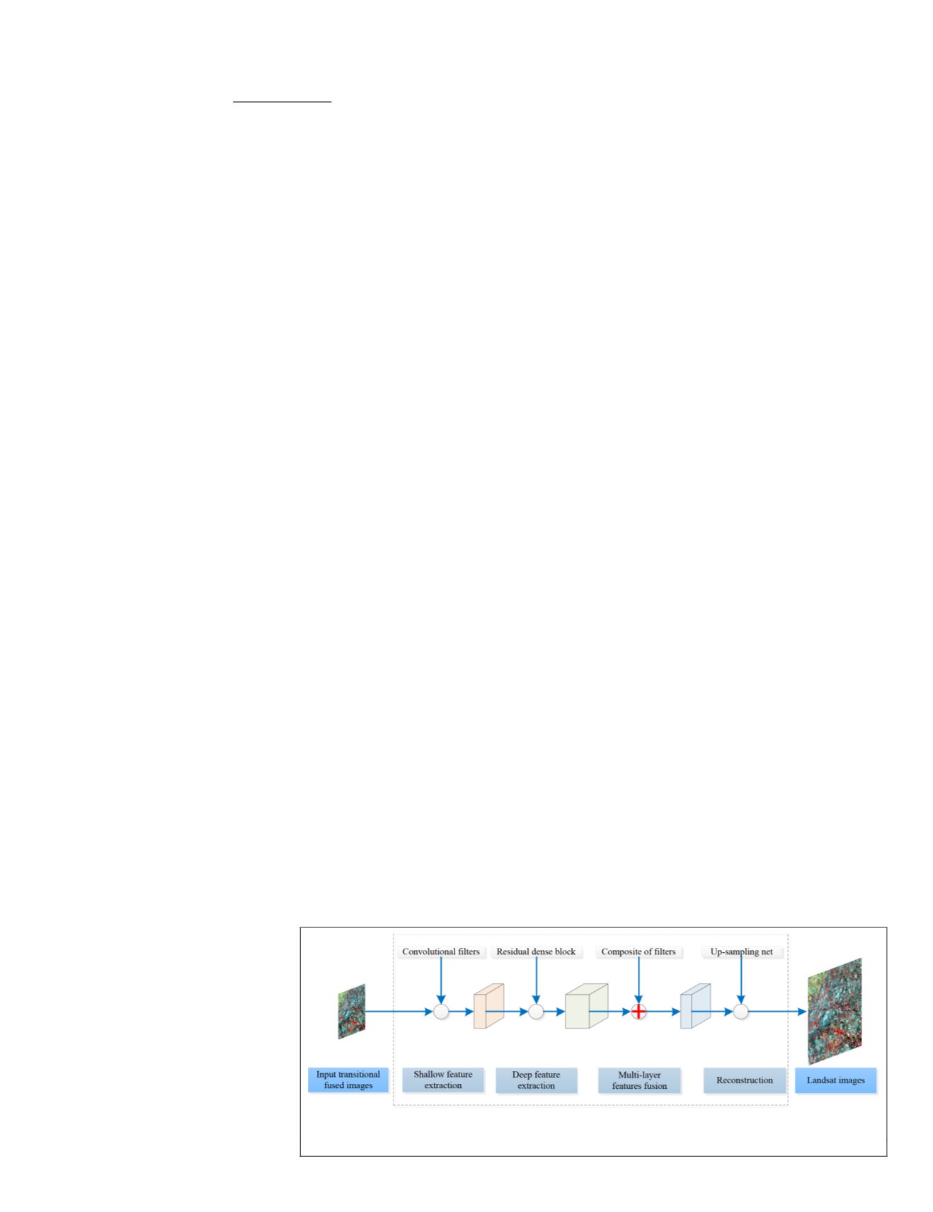
The network mainly consists four parts as shown in Figure
2. Firstly, two convolution layers are used to extract shallow
features from low-resolution images, and then residual dense
blocks (
RDBs
) are used to extract deep features. Thirdly, dense
feature fusion (
DFF
) is used to fuse the multilevel features ex-
tracted from previous layers. Finally, an up-sampling network
is used for super-resolution reconstruction to obtain high-res-
olution images. Next, we will introduce the network in detail.
Shallow Feature Extraction
Two convolution layers are used for shallow feature extrac-
tion (
SFE
) from low-resolution image
I
LR
. The features extract-
ed from two layers can be respectively formulated as
F
–1
=
H
SFE1
(
I
LR
);
(3)
c
=
H
SFE2
(
F
–1
);
where
H
SFE1(·)
and
H
SFE2(·)
represent the fir
convolutional layer, respectively.
F
–1
an
of these two convolution operations, respectively.
Deep Feature Extraction
Then, the extracted shallow feature
F
0
is used as the input of
the first residual dense block. After going through D residual
dense blocks, the hierarchical features
F
d
are extracted, and it
can be represented as
F
d
=
H
RDB,
d
(
F
d
–1
) =
H
RDB,
d
(
H
RDB,
d
–1
( … (
H
RDB,1
(
F
0
)) … ))
(5)
where
H
RDB,
d
can be a compos-
ite function of convolution and
rectified linear units (
ReLU
), it
represents the dth
RDB
.
Multilayer Features Fusion
To fully use the features extract-
ed from all the preceding layers,
the
DFF
is further conducted with
two operations. Firstly, the global
feature fusion (
GFF
) is used to
fuse multilevel features extracted
from residual dense blocks 1, …,
D. The adding of
GFF
can effec-
tively improve the performance
of the network and shows the benefits to stabilize the training
process, which has been demonstrated through quantitative
and visual analyses (Zhang
et al.
2018). The output
F
GF
can be
formulated as
F
GF
=
H
GFF
([
F
1
, … ,
F
D
])
(6)
where
H
GFF
is a composite function of a set of convolution op-
erators. The size of the convolution layer can be set to 1 × 1 or
3 × 3. The convolutional layer with the size of 1 × 1 can fuse
the multilevel features, and the 3 × 3 layer is used to further
extract features (Ledig
et al.
2017).
Then, the output feature
F
GF
and the shallow feature
F
–1
ex-
tracted from the first convolutional layer are fused to conduct
global residual learning to obtain the global dense feature
F
DF
,
F
DF
=
F
–1
+
F
GF
.
(7)
Super-Resolution Reconstruction
The extracted multilevel features from preceding layers are in
the low-resolution space. An up-sampling net in the high-
resolution space is introduced to reconstruct the final high-
resolution image
I
SR
.
I
SR
=
H
RDN
(
I
LR
),
(8)
where
H
RDN
represents the composite function of residual
dense network.
Experiments and Results
In order to assess the effectiveness of the proposed method,
its performances are analyzed and compared with
STARFM
and
Fit-FC
. Two different commonly used Landsat-
MODIS
data sets
are selected to test the effectiveness of the proposed method.
The two data sets are characterized by phenological and land-
cover type changes, respectively (Emelyanova
et al.
2013).
In the two experiments, most of the parameters settings in
the residual dense network are referring to the original paper
(Zhang
et al.
2018), the convolutional size is set as 1 × 1 for
local and global feature fusion, the size of all other convolu-
tion layers are set to 3 × 3, the number of filters is 64, all of
ns are
ReLU
(Nair and Hinton 2010), and
d using Adam optimizer. All algorithms
Xeon
CPU
Gold 6134 at 3.20 GHz and
GPU Tesla P100 16
GB
.
Data Set Introduction
The first study area is located in the Coleambally Irrigation
Area (
CIA
), south of New South Wales, Australia (34.0034°E,
145.0675°S). There are 17 cloud-free Landsat-
MODIS
image
pairs in the summer growing season of 2001–2002. All Land-
sat images in this area are from Landsat
ETM+
, covering 2193
km
2
, and the data set has six bands. The size of the image area
is 1720 × 2040 pixels with the resolution of 25 m.
Figure 2. The structure of residual dense network.
PHOTOGRAMMETRIC ENGINEERING & REMOTE SENSING
December 2019
909


