sets of edges delineated using
MESs
made with different win-
dow sizes to assess the impact of
MES
window size on edge
delineation. Tested window sizes ranged from 1 m × 1 m to 10
m × 10 m in steps of 1 m. The lower limit was selected based
on preliminary tests showing that window sizes smaller than
1 m × 1 m were ineffective at discerning physical structures
larger than approximately 1 m
2
. This value coincides with the
minimum area for which an aggregation can be considered
reef-like (Rabaut Vincx, and Degraer 2009). Conversely, the
upper limit was restricted by processing power.
Aggregation boundaries were defined as the base of the
slope that coincides with the transition between bare sedi-
ment and the mounds formed by
L. conchilega
(see Borsje
et
al.
2014). As such, relative elevation was assessed and values
at the base of the slope were selected. Selection was per-
formed by isolating elements of positive elevation from
LRMs
,
applying noise reduction through morphological filtering (i.e.,
erosion and dilation consecutively) of 3 cm, and extracting
the 0 m contour line which reflects deviations from the mean
elevation (i.e., neighborhood trend). Accuracy was evalu-
ated by assessing concordance between automatically and
manually delineated edges on data subsets from April 2014,
October 2014, April 2015, and August 2015. Concordance was
estimated by calculating inter-rater agreement (i.e., Cohen's
Kappa coefficient) between manual and automatic pixel as-
signment (Foody 2002).
Results
Acquisition, Processing, and Reconstruction
Mapping, processing, and photogrammetric reconstruction
had a success rate of 60% with twelve
DEMs
being produced
from 20 sets (i.e., one set per campaign): June, July, October,
and December 2013; March, April, June, July, August, and
October 2014; April and August 2015. Average coverage was
2488 m
2
(standard deviation [SD]: 759 m
2
) from an approxi-
mate total area of 3700 m
2
(i.e., 67% coverage). Average final
spatial resolution per pair was 2.98 mm·pixel
−1
(SD: 0.74
mm·pixel
−1
), with an average
RMSE
of 0.89 m (SD: 0.66 m) and
precision of 0.01m (SD: 0.02 m). Unsurprisingly,
RMSE
were
higher for reconstructions georeferenced using the Garmin
r (i.e., 1.30 m; SD: 0.35 m) in compari-
georeferenced using the
RTK GNSS
D: 0.04 m). Reconstruction artefacts
were found in six
DTMs
: October 2013, December 2013, March
2014, October 2014, April 2015, and August 2015. These
consisted of linear slopes that contrast with expected relief
abrupt changes in the interpolated height field. In addition,
artefacts associated to water presence as well as marked
differences in light conditions (i.e., brightness and contrast)
were identified on four orthophoto mosaics—October 2013,
June 2014, August 2014, and August 2015.
Semiautomated Detection
The accuracy of supervised maximum likelihood classifica-
tion in correctly identifying
L. conchilega
presence was on
average 70.0% (SE: 6.69; n = 12) per orthomosaic, ranging
from 23.1% for April 2015 to 97.6% for June 2014. Its ability
to correctly identify its absence was 83.6% (SE: 9.9%; n = 12),
ranging from 66.7% for August 2014 to 96.6% for June 2014.
Agreement between visual identification and
MLC
was very
low with Cohen’s Kappa ranging from −0.21 to 0.12. The clas-
sification procedure detected
L. conchilega
presence during
all campaigns with highest true presence percentage during
June and July of each year, coinciding with the recruitment
moment for that year (Alves
et al.
2017). The lowest estimate
was found on April 2015 for which visual inspection of ortho-
photo mosaics revealed high interspersion of sand within
L.
conchilega
aggregations (Figure 2).
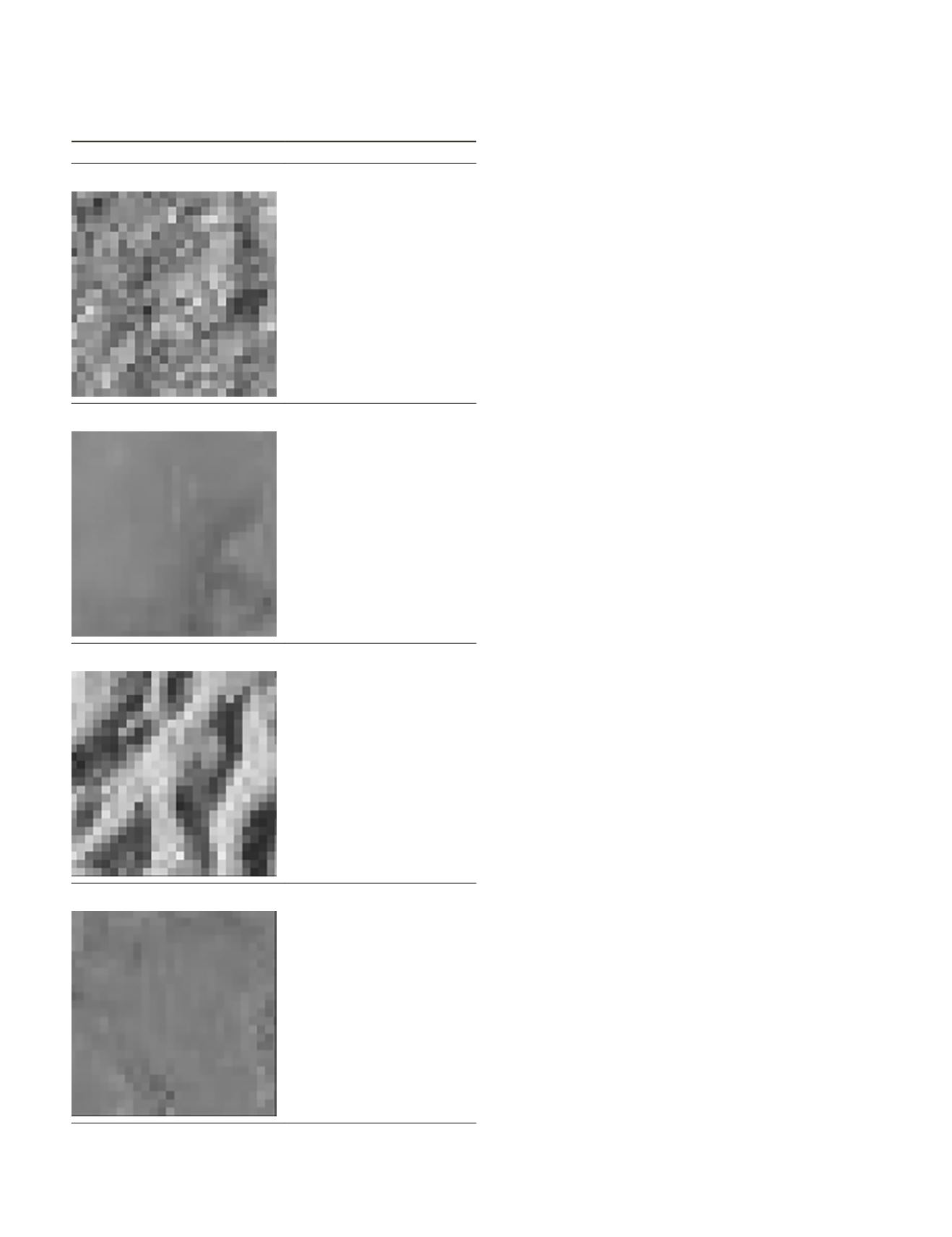
Table 1. Characterization of landscape features used to
generate class signatures for supervised maximum likelihood
image classification with example samples (each sample
corresponds to 25 cm × 25 cm).
Class
Description
Lanice conchilega
Biogenic structures composed
by L. conchilega tubes
characterized by shades of
brown with high variability in
color intensity.
Muddy sediment
Sediment characterized by light
brown colors with moderate
variability in color intensity.
Dry sand
Sediment characterized by grey
color of low variability in color
intensity.
Reworked sediment
Sediment characterized by
grey colors displaying marks
of reworking (i.e., wet sand,
resurfaced anoxic sediment,
visible grey sediment in
shallow water pools).
PHOTOGRAMMETRIC ENGINEERING & REMOTE SENSING
December 2019
901


