The segmentation results of
FNEA
at scales 40 and 50 are
shown in Plate 4 for further method comparison and to clarify
the features and advantages of the refined method. At these
scales, the segments of the man-made objects, including
buildings and roads, are basically similar to those in Plate
1 in terms of size. In a previous study (Wang and Li, 2014),
comprehensive comparisons were performed both qualita-
tively and quantitatively; the results show that
HBC-SEG
has
many advantages over
FNEA
. In the current study, we mainly
focused on visual interpretation of the performances of the
refined method and
FNEA
. The refined method was found to
better than
FNEA
in terms of
OP
boundary precision because
it inherited the advantage of edge constraint from
HBC-SEG
.
FNEA
exhibited the obvious co-existence of under- and over-
segmentation errors at relatively large scales. For example, at
scale 50, numerous over-segmentation errors still existed in
many man-made objects, including the building boundary in
Plate 4f and inner roads in Plate 4g and 4h. However, a large
amount of over-merging occurred at this scale. In Plate 4f, the
upper part of the building was merged with the neighboring
grassland. In Plate 4g, the cars were merged with the zigzag
lines. In Plate 4h, the building’s roof was dissolved into the
roads. These errors were caused by the global unique scale
parameter of
FNEA
. Controlled by the straight-line constraint
and threshold
T-SL
, only
IPSL
-neighbors in the refined method
were merged; hence, over-merging was avoided, and over-
segmentation errors were further reduced.
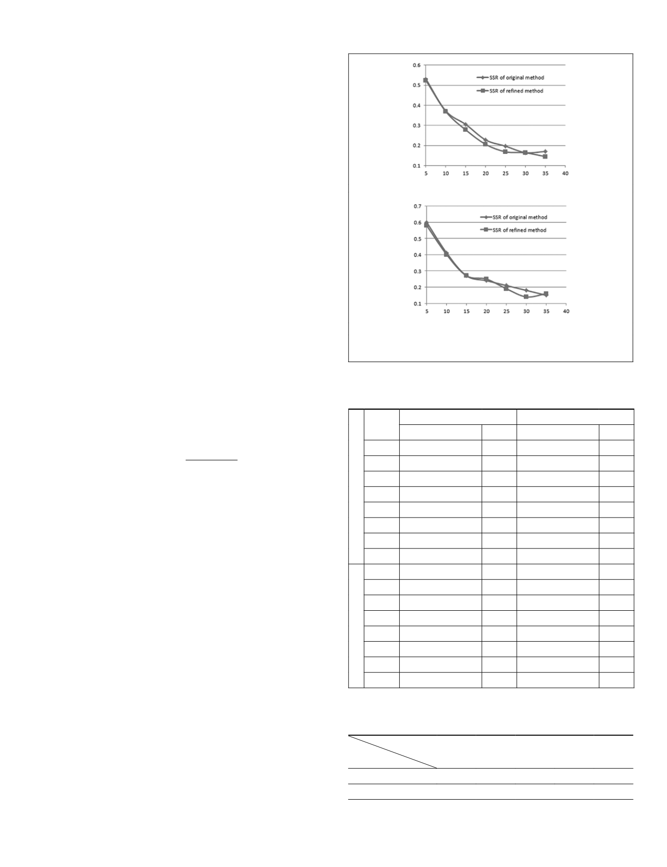
Scale-Parameter Dependency
Over-segmentation was further suppressed because of the
straight-line constraint. The refined method exhibited lower
dependency on the scale parameter than the original method.
The result was verified by segmentation shrinking ratio (
SSR
)
analysis, which has also been employed in previous literature
(Wang and Li, 2014).
SSR
is defined as follows:
SSR
s,ds
=
N N
N
s
s ds
s
−
+
,
(14)
where
s
denotes the scale,
ds
is the scale increment, and
N
s
and
N
s+ds
are the segment numbers at scales
s
and
s
+
ds
. This
index measures the decreasing ratio of the segment numbers
with some scale increment for a multi-scale segmentation
method. A small value means stable segment numbers during
merging from a small scale to a large one, i.e., segmentation is
insensitive to scale changes.
We changed scales from 5 to 40, calculated the
SSR
values,
and drew the curves for the two experimental areas (Table
3 and Figure 3). The curves of the refined method are below
those of the original method. The scale input had minimal
influence on the merging process as reflected by the
SSR
curves because more over-segmented segments are re-merged
to relatively larger scales in the refinement step.
Method Efficiency
Several different-sized remote sensing images were clipped to
test the efficiency of the methods. The results are presented
in Table 4. Before the refinement step, the segments were ad-
equately merged; thus, the number of segments that required
re-merging was relatively small. The experiments show that an
average of six iterations are necessary for the refinement step,
with
T_SL
equal to 50. Unlike in the original
HBC-SEG
, calculat-
ing the segment-line topology in the refinement step is time
consuming. The calculation depends on a number of segments
and straight lines, and recalculation is required during itera-
tive merging. Algorithm optimization can improve method ef-
ficiency by involving a spatial index and parallel computation.
(a)
(b)
Figure 3. SSR curves for the two experimental areas: (a) Area 1,
and (b) Area 2.
T
able
3. S
cale
D
ependency
A
nalysis
. T
he
ssr
V
alues
of
the
R
efined
M
ethod
in
A
rea
1
are
A
ll
S
maller
than
T
hose of
hbc
-
seg
; I
n
A
rea
2, F
ive of
the
S
even
ssr
V
alues
of
the
R
efined
M
ethod
are
S
maller
than
or
E
qual
to
T
hose
of
hbc
-
seg
Area 1
Scales
HBC-SEG
Refined method
Segment number SSR Segment number SSR
5
9883
0.53
7993
0.52
10
4640
0.37
3803
0.37
15
2913
0.31
2400
0.28
20
2024
0.23
1734
0.21
25
1563
0.20
1376
0.17
30
1255
0.17
1144
0.16
35
1048
0.17
956
0.15
40
869
/
817
/
Area 2
5
6671
0.60
5663
0.58
10
2657
0.41
2362
0.40
15
1561
0.27
1422
0.27
20
1139
0.24
1038
0.25
25
869
0.21
778
0.19
30
685
0.18
633
0.14
35
560
0.15
543
0.16
40
474
/
457
/
T
able
4. M
ethod
E
fficiency
. T
he
M
ethods were
T
ested
on
the
S
ame
P
latform
by
S
etting
T
he
S
cale
P
arameter
(C
onstantly
)
to
a
S
mall
V
alue
of
10; T
he
T
ime
U
nit
is
in
S
econds
,
and
the
I
mage
S
ize
is
in
P
ixels
Image size
Method
256
×
256
512
×
512
1024
×
1014
2048
×
2048
4096
×
4096
HBC-SEG
2
5
10
66
272
The refine step
2
3
36
94
412
PHOTOGRAMMETRIC ENGINEERING & REMOTE SENSING
May 2015
405


