training data set (
C
,
y
) is con-
structed to train the discriminative
model-
GP
. Our task is labeling a
new coming video clip
c
* to a traf-
fic state with the highest probabil-
ity
P
(
y
*|
C
,
y
,
c
*)
For simple illustration the
binary classification with two traf-
fic states
y
t
∈
{–1, +1} is considered
here. The binary classification is
easily extended to multiple classifi-
cation by using the one-against-all
or one-against-one strategy.
The general formulation of prob-
ability prediction for a new test
sample given the training data (
C
,
y
)
under a
GP
model is:
p
(
y
*=+1|
C
,
y
,
c
*)=
∫
p
(
y
*|
f
*)
p
(
f
*|
C
,
y
,
c
*)
df
*,
(24)
where
p
(
f
*|
C
,
y
,
c
*) is the distribution of latent variable
f
t
cor-
responding to sample
c
*. It is obtained by integrating over the
latent variable
f
=(
f
1
, …,
f
T
):
p
(
f
*|
C
,
y
,
c
*)=
∫
p
(
f
*|
C
,
y
,
c
*,
f
)
p
(
f
|
C
,
y
)
d
f
(25)
where
p
(
f
|
C
,
y
)=
p
(
f
|
y
)=
p
(
f
|
C
) (/)
p
(
y
|
C
) is the posterior over
the latent variables.
p
(
y
|
C
) is the marginal likelihood (evi-
dence),
p
(
f
|
C
) is the
GP
prior over the latent function, which
in
GP
model is a jointly zero mean Gaussian distribution and
with the covariance given by the kernel K.
The non-Gaussian likelihood in Equation 25 makes
the integral analytically intractable. We have to resort
to either analytical approximation of integrals or Monte
Carlo methods. Two well known analytical approximation
methods are very suitable for this task, namely the
La-
place
[williams1998bayesian] and the
Expectation Propaga-
tion
(EP) [minka2001family]. They both approximate the non-
Gaussian joint posterior as a Gaussian one. In this paper we
adopt the
Laplace
method since its computation cost relative
lower than EP with comparable accuracy. As introduced in
[26]
,
the mean and variance of
f
* are obtained as follows:
p
(
f
*|
C
,
y
,
c
*)=
N
(μ*,
σ
*),
(26)
with
μ*=
k
(
C
,
c
*)
T
K
–
f
,
(27)
σ
*
2
=
k
(
c
*,
c
*)–
k
(
C
,
c
*)
T
(
K
+
W
–
)
k
(
C
,
c
*).
(28)
where
W
Δ
= –
∇∇
log
p
(
y
|
f
) is diagonal.
K
denotes a
T
×
T
covariance matrix between
T
training points.
k
(
C
,
c
*) is a
covariance vector between T training video clips
C
and test
clip
c
*, while
k
(
c
*,
c
*) is covariance for test clip
c
*, and
f
= argmax
f
p
(
f
|
C
,
y
). Given the mean and variance of latent
variable
f
* for test clip
c
*, we compute the prediction prob-
ability using Equation 24.
The covariance function and its hyper-parameters
Θ
cru-
cially affect
GP
models performance. The Gaussian radial basis
function (
RBF
) is one of the most widely used kernels due to
its robustness for different types of data and is given as below:
K
RBF i j
i
j
c c
c c
,
(
)
=
−
−
σ
2
2
2
2
exp
N
(29)
Θ
=[
σ
,
l
] is the hyper-parameter set for
RBF
. We optimize the
hyper-parameters using Conjugate Gradient method
[27]
.
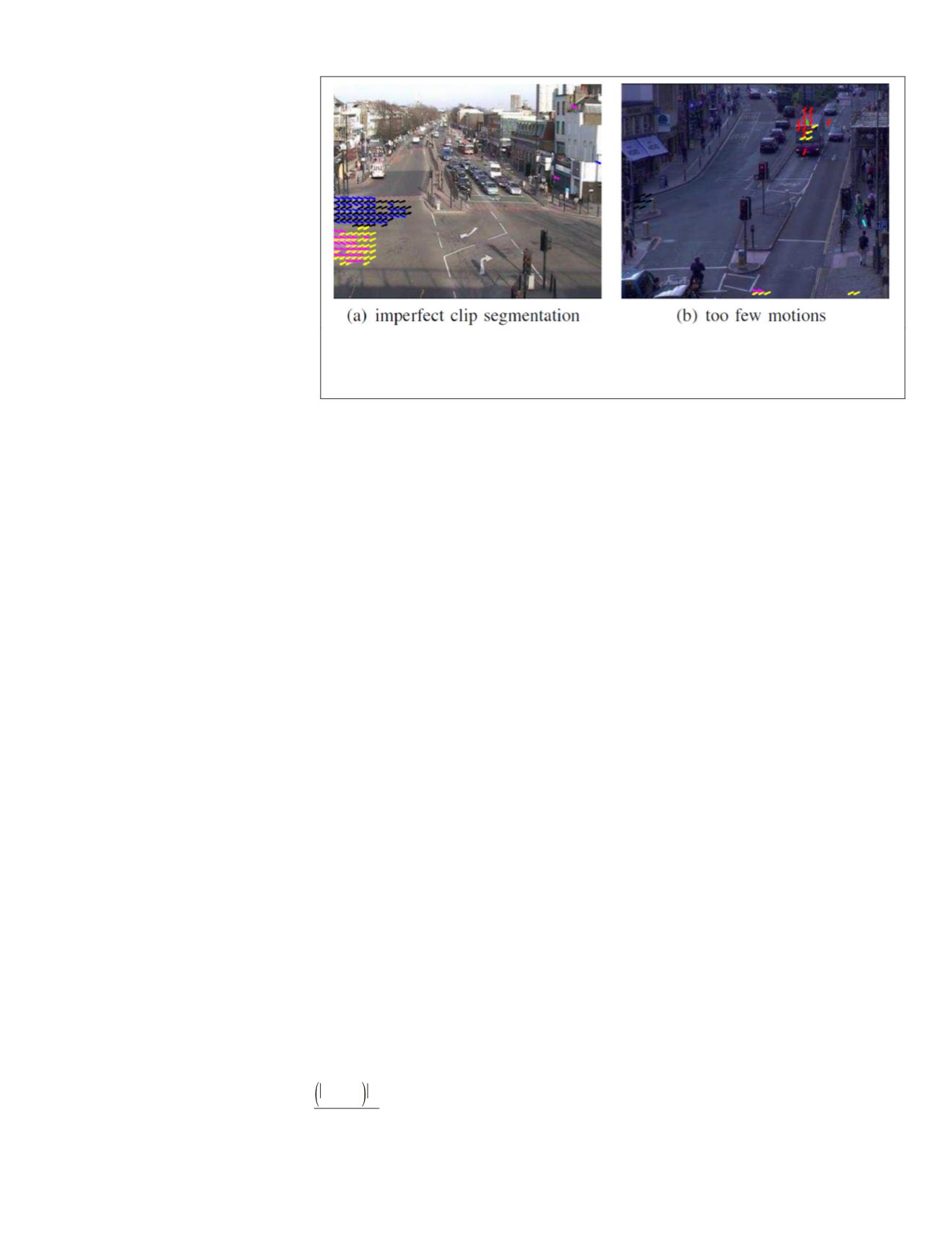
Integration of Transition Information into GP Classifier
The input video is segmented into clips along time. It cannot
be ensured that each clip is precise in a traffic state interval.
In practice, sometimes the transition of two states occur in a
clip, as shown Figure 5a In the other cases, the scene is silent
in some clips: there are very few motions, as shown Figure 5a.
In these two cases, the
GP
classifier is hard to exactly classify
the states. Fortunately, a crowded traffic scene is normally
regulated by traffic lights. The transition between two traffic
states is rule-based, e.g., the transition from state Figure 7a to
state Figure 7c is impossible. The transition information from
the Learning states using the
HDP
-
HMM
Section makes signifi-
cant sense here.
Figure 5 shows examples of confused traffic states: (a)
Imperfect segmented clip may contain motion information
belonging to different states, and (b) A silent clip contains too
few useful motion information. Both of these two cases make
the system hard to determine the right state.
We define a state energy for clip
t
as follows:
E
(
y
t
=
s
i
|
y
t
–1
=
s
j
) =–log{
p
(
y
t
|
c
t
)}
(30)
+
β
log{
m
s
i
,s
j
} (1–
δ
(
y
t
y
t
–1
))
y
t
=argmin
y
t
=
s
t
E
(
y
t
|
y
t
–1
)
(31)
where
p
(
y
t
|
c
t
) is the likelihood of the
t
th
clip labeled as state
s
i
given by Equation 24:
m
s
i
,s
j
is the transition probability from
state
s
j
(state of last clip) to
s
i
, and
δ
(
y
t
y
t
–1
)=1,
if y
t
=
y
1
,
else
0.
β
is the weight of transition energy and is set experimentally as
0.1. It means that, if the state does not change, we do not need
to care about the transition problem. If the transition of the
states happens, we will take the transition information into
account and choose the state which has minimal state energy.
Abnormal Events Detection
Abnormal events identification is always one of the most
interesting and desired capabilities for automated video be-
havior analysis. However, dangerous or illegal activities often
have few examples to learn from and are often subtle. In other
words, it is a challenging problem for identifying abnormal
events according to their motion patterns for supervised clas-
sifier. To tackle this problem, the abnormal events should be
defined at first. They are roughly categorized into three groups.
Figure 5. Examples of confused traffic states: (a) Imperfect segmented clip may contain
motion information belonging to different states, and (b) A silent clip contains too few
useful motion information. Both of these two cases make the system hard to determine
the right state.
PHOTOGRAMMETRIC ENGINEERING & REMOTE SENSING
April 2018
207


