β
~
GEM
(
γ
),
(16)
τ
k
~
DP
(
α
,
β
),
(17)
ϕ
k
~
H
(18)
y
t
|
y
t
–1
~
Multi
(
τ
y
t
–1
),
(19)
x
t
|
y
t
=
s
i
~
Multi
(
ϕ
s
i
),
(20)
where
y
t
S
={
s
i
,…,
s
N
S
} is the state of the
i
th
clip and
S
is the set of
possible states and
N
S
is the total number.
x
t
is the observation set
(visual words). In this case, each vector
τ
k
={
τ
kl
}
I=1
…
L
is one row of
the Markov chain’s transition matrix from state
k
to the other states
and
L
is the number of states. For a better illustration, we denote
these transition matrix as
M
= {
m
i,j
}
i,j
=
1
…
L
throughout this paper.
Given the state
y
t
, the observation
x
t
is drawn from the mixture
component
ϕ
s
i
indexed by
y
t
. Gibbs sampling schemes are applied
to do inference under this
HDP
-
HMM
. Figure 7 shows the typical
traffic states learned by
HDP
-
HMM
for
QMUL
Junction Dataset
[8]
.
The same as the activity learning using
HDP
model, the traf-
fic states learned by
HDP
-
HMM
also involve some unexpected
results. The typical traffic states are selected in the similar
way as previously described in this Section.
Representation of Activities and Video Clips
Activity Representation
Each activity
θ
k
is characterized by a multi-nominal distribu-
tion {
ϕ
k
} over the words in codebook. The probability of
i
th
word in activity
θ
k
is denoted as
p
kx
i
and
p
k
kx i
N
i
x
x
p
=
{ }
=
1
,
p
kx
i
N
i
x
=
=
∑
1
1
and
N
x
is the size of codebook. Similar to the
operation previously described which selects the representa-
tive activity, we also select the representative visual words to
represent each activity in the same way:
p
k
x
is sorted in de-
scending order
p
′
k
x
= {
p
′
kx
1
≥
…
≥
p
′
kx
x
}, and then the accumulated
sum of probability is calculated as:
′ = ′
=
∑
P
p
kj
kx
i
j
i
1
(21)
those visual words which satisfy :
w
θ
k
= {
x
j
|
P
′
kj
≤
0.9}
(22)
are chosen to represent activity
θ
k
. It is the set of the most
frequently co-occurring words in the same activity. The words
falling into the rest 10 percent are viewed as noise or rare
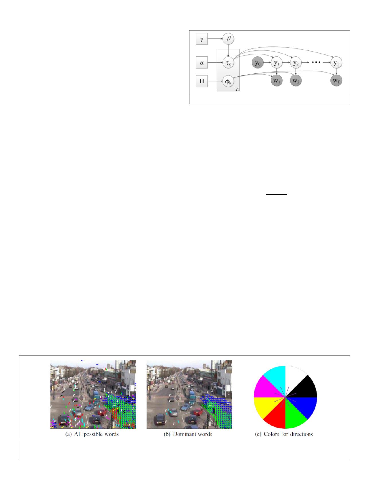
motion. Figure 4 shows a comparison between all possible
co-occurring visual words and the selected representative
words in the activity of vehicles driving downward.
Video Clip Representation
Feature vectors of activities from last step are variant in length
because the number of representative words of different activi-
ties is unexpected. They are not suitable to be used to describe
a video clip directly. We construct a feature vector to explain a
clip using learned activities in a new way as follows.
x
t
ti i
N
x
x
=
{ }
=
1
denotes that there are
N
t
the words present in
clip
t
totally.
x
t
is compared with each activity word set
w
θ
k
and the percentage of intersection is calculated as:
p
N
tk
t
k
a
t
=
∩
x w
(23)
It explains the proportion of activity
θ
k
in this clip. The
feature vector which explains what happens in this clip is
represented as
c
t
={
p
t
1
, …,
p
tk
}, as shown in Figure 7 (e) to (h).
Figure 4 is a comparison between the activity pattern
before and after filtering the unnecessary words. The vi-
sual words in the left part of image (a) seem chaotic and are
filtered out. In Figure 4b, the activity is represented better by
the selected visual words. The color of the arrow denotes the
quantified motion direction, as illustrated in Figure 4c.
Traffic States Classification
In this section, we first discuss how to use
GP
models to clas-
sify traffic states in a newly screened video. Then, we inte-
grate the transition information learned by
HDP
-
HMM
with
GP
model to enhance the classification accuracy.
Gaussian Process for Classification
The
HDP
-
HMM
has mined the main traffic states
S
from training
video sequence and each training video clip is labeled with
a state label
y
t
∈
S
, where the subscript
t
is the clip index.
c
t
}
is the feature vector of clip
t
given by Equation 23. Now the
Figure 3. A graphical representation of the
HDP-HMM
model.
Figure 4. A comparison between the activity pattern before and after filtering the unnecessary words. The visual words in the
left part of image (a) seem chaotic and are filtered out. In (b), the activity is represented better by the selected visual words.
The color of the arrow denotes the quantified motion direction, as illustrated in (c).
206
April 2018
PHOTOGRAMMETRIC ENGINEERING & REMOTE SENSING


