percentage among all training clips, as illustrated in Figure 7a
to 7d, and their corresponding average feature vectors in the
training video shown in Figure 7e to 7h. Figure 7i is the state
transition graph with transition probabilities and directions.
They are explained as follows
• Vertical flow: Activities 1 and 2 dominate in this interac-
tion. The activities topics such as 5, 8, and 10 related to
vertical traffic activities have also relative high values in
the histogram.
• Leftward flow: It is absolutely dominated by topic 3. Ac-
tivities 7, 12, 17, and 19 are also important components.
The feature values of activities 11, 17, and 22 are relative
high because of pedestrians.
• Rightward flow: It mainly consists by activities 4, 6, and
10. Activities 1, 8, and 9 overlap this flow. The feature
values of activities 15 and 18 are relative high because of
pedestrians.
• Left and right turn: This state happens during the state of
vertical flow, when the vertical flow temporally termi-
nates. It is a complicated interaction among a couple of
topics, such as activities 1, 3, 6, 7, 8, and 12.
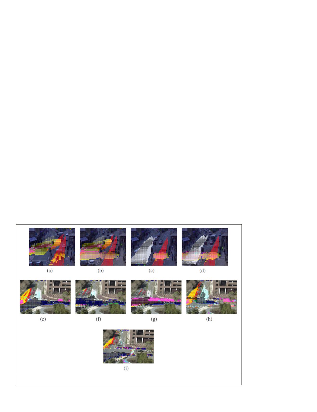
Figure 8 shows typical traffic states learned by
HDP
-
HMM
model for
QMUL
Junction Dataset 2 (8a) to (8d) and MIT Data-
set (8e)to (8i).
The learned typical traffic states in
QMUL
Junction Dataset
2 are shown in Fig8a to 8d, and the states of MIT Dataset are
shown in Figure 8e to 8i.
QMUL
Junction Dataset 2 has two
main flows and 4 typical states: vehicles driving vertical with-
out (Figure 8c) or with (Figure 8d) pedestrian; vehicles making
a turn at the crossing without (Fig8a) or with (Figure 8b). The
traffic scene in MIT Dataset is relative less busy and interac-
tive than the first
QMUL
scene: Figure 8e explains a vertical
flow. Vehicles from bottom may make a left turn; Figure 8e
explains a rightward flow and vehicles making a left turn and
driving upward; Figure 8g explains a horizontal flow in two
directions. Vehicles may make a left turn in this state; Figure
8h explains vehicles driving downward from top and pedes-
trian crossing the road; Figure 8i illustrates that, vehicles stop
behind the crosswalk and pedestrian cross the road.
Traffic States Recognition
The
GP
classifier was firstly trained with learned activities and
states. The screened video sequence was segmented into clips
of 75 frames each.
Our experimental results are compared with the other
popular methods: Dual-
HDP
model
[9]
, Markov Clustering Topic
Models (
MCTM
)
[8]
,
LDA
and
HMM
. They adopted diverse length
of video clip ranging from 1 second to 10 seconds. The experi-
mental results are directly cited from
[19]
(for
QMUL
Dataset)
and
[9]
(for MIT Dataset). From the comparison in Table 1, we
see that our model outperforms other three popular meth-
ods in terms of classification results in the
QMUL
Dataset. In
contrast to the Dual-
HDP
model in the MIT Dataset as listed
in Table 2, our methods also achieved better classification re-
sults. Furthermore, Dual-
HDP
model is a batch processing. To
validate our method, we have executed one more experiment
in the
QMUL
Junction Dataset 2. The results is listed in Table 3.
It is worth point out that some clips were falsely recog-
nized by traditional
GP
classifier and corrected by our model.
For example, it is ambiguous to determine whether the state
in Figure 8e belongs to state Figure 8e or Figure 8f only based
on its appearance. It was falsely classified as the second one
with higher probability by
GP
classifier. Because its previous
clip is in the state as Figure 8e, it is successfully corrected by
using transition information, as described in the Integration of
Transition Information into
GP
Classifier Section.
Anomaly Detection
Then, the proposed framework’s performance of detecting the
abnormal events previously defined is evaluated in each data-
set. In the scene of
QMUL
Junction Dataset, the main abnormal
events include Jaywalking, illegal U-turns and emergencies
caused by ambulanc-
es, fire engines and
police cars. Figure
10 illustrates two
detected abnormal
events caused by
rarely occurring
motions in the
QMUL
Junction scene. For
instance, the ambu-
lance is driving in an
absolutely forbidden
direction in the lane,
whose motions have
never occurred in the
training data (Figure
10a).
Figure 9 shows
examples of abnor-
mal events caused by
rarely occurring mo-
tions. In the training
dataset such motions
have rarely or never
occurred. They do
not belong to any
typical activities. The
red boxes highlight
the abnormal agents.
Figure 10 shows
examples of abnor-
mal event caused
Figure 8. Typical traffic states learned by
HDP-HMM
model for
QMUL
Junction Dataset 2 (a) to (d) and
the
MIT
Dataset (e) to (i).
210
April 2018
PHOTOGRAMMETRIC ENGINEERING & REMOTE SENSING


