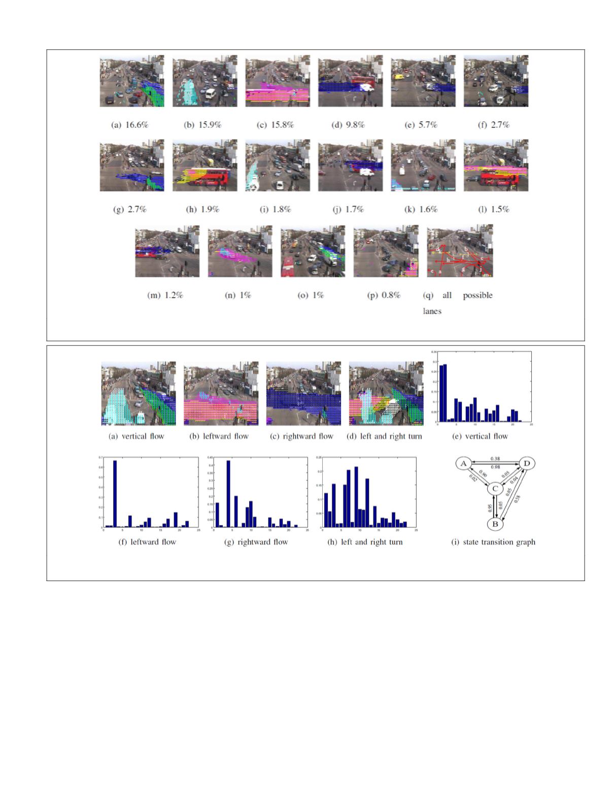
painted and marked with alphabetic letters in Figure 6q. They
are explained as follows:
• Flow a and b: vehicles driving in vertical directions, con-
sists of activities 1, 2, 13, etc.
• Flow c and e: vehicles making a left turn and driving out
of the scene. It can be explained by activities 6, 20, and
16, respectively.
• Flow d: vehicles turning left from the left entrance. It is
explained by the upper part of activity 4.
• Flow f and g: vehicles making a right turn in the middle
of the junction during the vertical flow, shown as activi-
ties 9 and 12.
• Flow h (leftward) and i: vehicles driving leftward and
part of them making a right turn. It is dominated by ac-
tivities 3, 17, and 19.
• Flow h (rightward) and j: vehicles driving rightward and
part of them making a right turn. It mainly consists of
activities 4, 6, 10, 15, and 18.
• Flow k, l and m: pedestrian crossing the road. Activities
15, 17, 18, and 22 show these behaviors.
For
QMUL
Junction Dataset 2 and MIT Dataset, 21 and 24 typi-
cal activities are learned respectively. Due to space constraint,
they are not shown and discussed here.
Figure 7a to 7d) are typical traffic states learned by
HDP
-
HMM
model and 7e to 7h) are their corresponding average
components of typical activities. Figure 7i is the state transi-
tion graph noted with transition probabilities and directions.
The
HDP
-
HMM
automatically learned 9 traffic states. 4 of
them are selected as typical states which have the highest
Figure 6. (a) to (p) Some dominant activities and their percentages discovered by HDP models; and (q) Manually labeled legal
vehicles driving lanes (red lines) and pedestrians walking lanes (yellow dashed lines).
Figure 7. (a) to (d) are typical traffic states learned by HDP-HMM model and (e) to (h) are their corresponding average
components of typical activities, and (i) is the state transition graph noted with transition probabilities and directions.
PHOTOGRAMMETRIC ENGINEERING & REMOTE SENSING
April 2018
209


