directly results from spatial processes operating at various
levels, higher
FD
occurs at the scale where more processes
operate. With
FDs
, the spatial processes performed at different
levels are measurable and results are thus comparable.
Fractal geometry has been employed for many purposes
in remote sensing including image classification (Chen
et
al.
, 1997; De Cola, 1989; De Jong and Burrough, 1995; Emer-
son
et al.
, 1999, and 2005; Lam, 1990; Lam and Quattrochi,
1992; Myint, 2003; Qiu
et al.
, 1999; Read and Lam, 2002;
Weng, 2003). However, its roles in classifying images have
not been fully explored. While fractals have proved to show
some promise in traditional
ML
image classification (Emer-
son
et al.
, 2005), most of such studies did not elaborate how
the selection of different input variables in terms of the data
(e.g., the image’s spectral bands) and algorithms (e.g., the size
of moving window and the algorithm used to measure
FD
values) in creating fractal features influences the classification
results. Among all these input variables, the size of moving
window dictated by the number of pixels, is the most critical
on texture-based image processing including those relating to
fractals, since it relies on the use of texture features that must
be extracted locally. While the traditional moving window
method remains a popular method to measure local texture
features, problems arise as how to effectively calculate local
FDs
with different window sizes. The choice of the optimal
window size has been long as to be elusive in all texture-
based image analyses and those based on fractals are not an
exception. Overall, to sufficiently extract characterized spatial
information for a given land cover, a large window is required
to produce stable textural measures. Yet it then increases the
potential of covering more land covers, which introduces
incorrect spatial information (Pultz and Brown, 1987), and en-
hances the edge effects, which is blamed for most of the clas-
sification errors (Maillard, 2003; Zhou and Lam, 2008). With
a detailed local variation, a small window size would help to
reduce the mixed pixel problem as well as the edge effects.
However, it often fails to capture
the particular patterns of most land
use and cover types and thus is
less able to produce stable textural
features. Additionally,
FD
values
are estimated with the regression
procedure that requires a minimum
number of cases, determined by the
underlying software, to guarantee
a statistically-acceptable regression
model. This places a bottom line
on the window size to measure
FDs
. Probably because of the diffi-
culty of identifying an appropriate
window size to produce suitable
fractal features, the use of
FDs
in
image classification has not been
extensive, particularly for large
study sites. Most previous image
classification studies where the use
of fractals is reported, the decision
related to the selection of the “ap-
propriate” window size for gener-
ating fractal feature is randomly
dictated by the research constraints
(Chen
et al.
, 1997; De Jong and Bur-
rough, 1995; Emerson
et al.
, 2005).
Very few of them have attempted to
provide an in depth analysis of the
relationships between this variable
and its influence on image classifi-
cation results in great details.
This research aimed to examine the potential of fractal
information in the supervised
ML
image classification of a
typical Midwest urban environment in the US using a Landsat
ETM+
imagery. The traditional
ML
algorithm was considered in
the study because it is still popular due to its fast computing,
easy implementation, memory efficient, and yet exhibiting
acceptable accuracy. Specifically, the objectives of the pres-
ent study were to (1) provide a critical survey of identifying
the optimal window size(s) for fractals-based texture feature
extraction, and (2) present a comprehensive evaluation of the
contribution of the fractals-based textural features in support-
ing separability analysis amongst classes and image classifica-
tion using the
ML
logic.
Study Area and Dataset Preprocessing
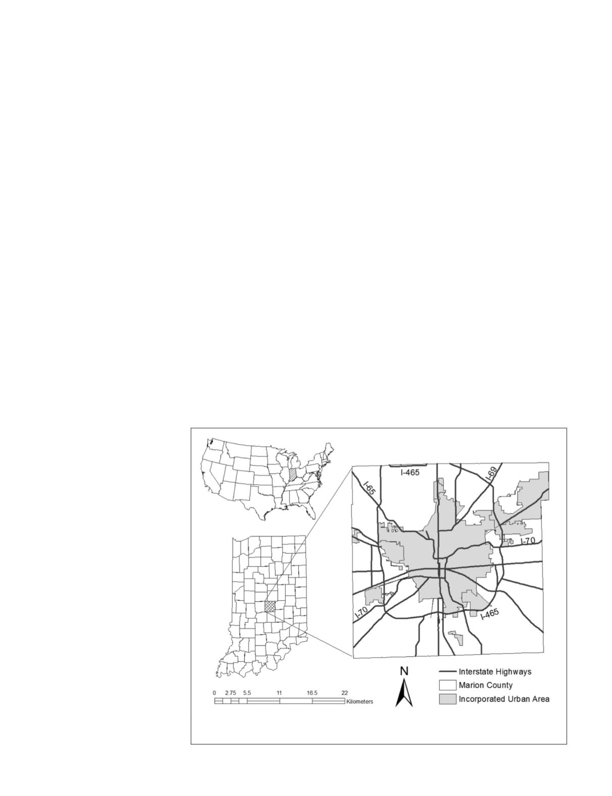
The study area is Indianapolis, located in Marion County,
Indiana, in the United States (Figure 1). With a consolidated
city-county structure (Nunn, 1995), the City of Indianapolis
and Marion County are often loosely considered the same.
The city has a total area of 963.5 square kilometers (98.14% of
land and 1.86% of water). With a total population of 829,718
(Census, 2010), Indianapolis ranks the nation’s 12
th
largest city
and is the geographical center of Indiana and the capital of
the state. With roads leading out of the city center at all direc-
tions, Indianapolis has been famous as “The Crossroads of
America”. Since the city is located on a flat plain (the Central
Till Plains) and is relatively symmetrical, it has the possibil-
ity to expand in all directions. Like many other cities in US,
its urban area enlarges at the expense of the loss of adjacent
agricultural areas and forestlands. Indianapolis is now the
most populous city of the state and the second most populous
Capital in the US.
A 30 m Landsat
ETM+
image taken on 22 June 2000 that has
been used in previous fractal-based studies (Liang
et al.
, 2013;
Liang and Weng, 2014) was applied in the current research.
Figure 1. A map of the study area: Indianapolis, Marion County, Indiana, (the gray area
shows the incorporated area boundary for the city).
696
November 2018
PHOTOGRAMMETRIC ENGINEERING & REMOTE SENSING


