critical
t
-value at the 0.05 signifi-
cance level for statistical inference.
Similarly, if the normal distribu-
tion assumption for the observed
data was not justified, a nonpara-
metric sign test was performed to
determine whether any significant
difference in the observations ex-
ists. If
p
is the probability that the
difference between the two datasets
is positive, and if the difference is
insignificant,
p
will take the value
0.5 (i.e., the difference is the same
about 50 percent of the time). Thus,
the hypothesis was to test:
H
0
:
p
=0.5
against
H
1
:
p
≠
0.5
For large samples,
(
.
under
;
H Z
n p
N
0
0 5
0 5 1 0 5
0 1
,
)
. (
. )
~ ( , )
=
−
−
ˆ
where
n
is the number of samples
and
p
ˆ is the proportion of positive
observations (Sheskin, 2003). The
computed
Z
-value is compared
with the critical
Z
-value at 0.05
significance level for a statistical
result.
Results
Analysis of the Stability of
Control Point Settings
A dataset consisting of 82 control
points was used for stability analy-
sis. This particular dataset was
located in Bannock County, Idaho
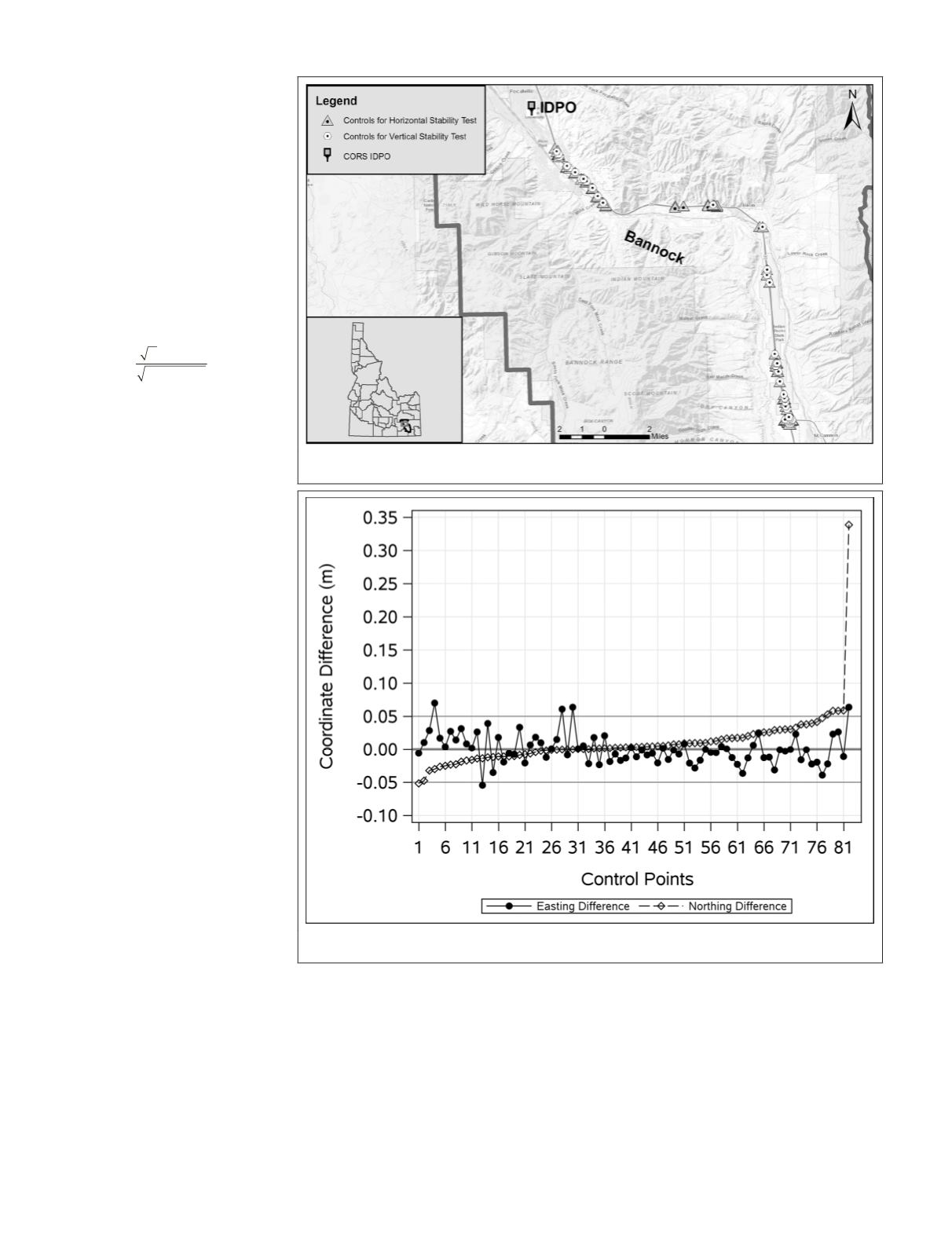
(Figure 1).
Analysis of Horizontal Coordinates
Horizontal components were col-
lected in
NAD 83
(1986). Data were
collected first in 2013 and then
again in 2015 by two different
surveyors and the Real-Time Kine-
matic (
RTK
)
GPS
technique was used
for both collection methods.
The difference in horizontal
components (i.e., the difference in
easting and the difference in north-
ing observed between 2013 and
2015) were analyzed to determine
correlation (Figure 2). This figure
was sorted by northing differ-
ence, so the abscissa indicates the
control point’s placement in the
sorting order and the ordinate is
the difference (in meters) between
observations from 2013 relative to
2015. The difference is confined to be within for most control
points tested. The 1
σ
reported for observations in both 2013
and 2015 was 3 cm. Most differences are well within
±
the 2
σ
standard deviation. Only one extreme difference in north-
ing is visible in the plot. Upon inspection, this control point
showed an easting difference of 6.3 cm (very near 2
σ
) suggest-
ing a data entry error for the northing value.
Histograms of differences are shown in Figure 3a. The
population is zero centered in both easting and northing dif-
ferences. To identify the possibility of outliers, boxplots were
produced (Figure 3b). The box spans from the 0.25 quantile to
the 0.75 quantile surrounding the median with whiskers that
extend to span the dataset excluding outliers. The box-whis-
ker plots indicate three probable outliers in easting and four
probable outliers in northing.
The normal distribution assumption was justified for east-
ing differences, and a
t
-test was performed to determine if the
difference between the eastings measured in 2013 and 2015
were significant (Table 1). The observed
t
-statistic was 0.18,
which was less than the critical
t
-value of 1.99 (
t
0.025,81
) at 5
percent significance level:
p
= 0.85 for a two-tailed compari-
son. Hence the null hypothesis is not rejected, and it was
Figure 1. Control points used for horizontal and vertical stability analysis located in
Bannock County, Idaho.
Figure 2. Differences in northing and easting between 2013 and 2015 control point
observations using
NAD
83(1986).
218
April 2018
PHOTOGRAMMETRIC ENGINEERING & REMOTE SENSING


