Q
i
=
A
i
N
–1
A
i
T
(10)
Given the error in coordinate measurements, the variance
of any point (
μ
,
ν
) in the line direction is:
σ σ
µ
σ
2
0
2
1 2
2
1 2
2
1 2
1 2
2 2
2
0
1
2
2
2
= +
+
(
)
+
(
)
⋅
+
+
(
)
⋅
⋅
p p h p p
v
p p
p p w m
2
(11)
If the
T
1
–
T
4
are deployed in a narrow belt area, that is
μ
/
(
wm
)>>2
ν
/
h
and
μ
/
wm
>>1, the standard deviation is approxi-
mated by:
σ
µ
µ
≈
+
+
⋅
⋅
p p
p p wm
1 2
1 2
0
2
(12)
For this reason,
T
1
–
T
4
are deployed in each corner of the
overlap area to minimize the variance. In this case, the vari-
ance of affine compensation depends on the lateral overlap.
With Equation 12, the standard deviation is linearly related to
the sample coordinate
μ
when the overlap is fixed.
After translating the coordinates into the
oμ
ν
system, the
cofactors of
T
5
–
T
8
are:
q q
p p p p
p m p
m
p p m
q
5 6
2
0
2
1 2 1 2
1
2
2
1 2
2
1
1
1
1
1 2
2
= = = +
+
+
+
⋅
⋅ −
(
)
+ ⋅ −
(
)
(
)
⋅
σ
σ
7 8
2
0
2
1 2 1 2
1 2 2
2 2
1 2
2
1
1
1
2
= = = +
+
+
+
⋅
+ − ⋅
(
)
⋅
q
p p p p
p p p m
p p m
σ
σ
(13)
For the first strip, only coordinate measurement errors
are taken into consideration. The weights are
p
1
=
p
2
=1, and
Equation 13 becomes:
q q
m
m
q q
m
m
5 6
2
7 8
2
1 5
2 3
4
1 5
2
4
= = +
−
(
)
= = +
−
(
)
.
.
(14)
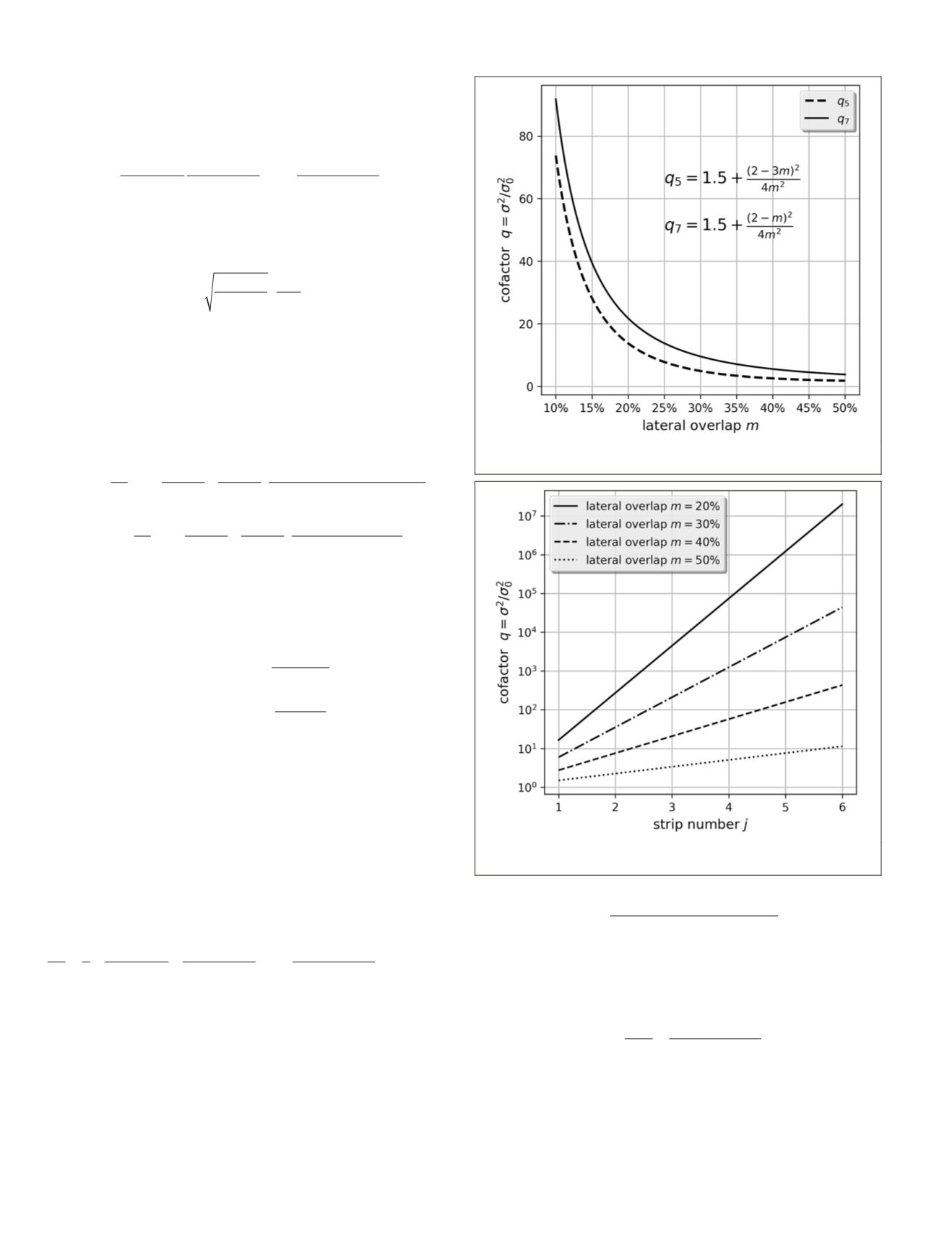
According to Equation 14, with the increase in overlap
from 0 to 50%, the geopositioning error decreases, as illus-
trated in Figure 3. The larger the overlap, the higher the ac-
curacy. If the overlap
m
is 20%,
q
5
and
q
7
are 13.75 and 21.75,
respectively. If the overlap
m
= 40%, the cofactors are 2.5 and
5.5. In theory, the theoretical precision of the adjacent scenes
in the same strip is in conformity with the same laws.
The standard deviation of sample
c
is slightly different from
that of line
r
because of the epipolar constraint (Pan, 2017). For
the along-track stereo images, the epipolar constraint halves
the measurement variance. Hence, the cofactor is:
σ
σ
µ
c
p p h p p
v
p p
p p w m
2
0
2
1 2
2
1 2
2
1 2
1 2
2 2
2
1
2
1
2
1
2
= +
+
(
)
+
+
(
)
⋅
+
+
(
)
⋅
⋅
(15)
with initial weights
p
1
=
p
2
= 2. A similar behavior could be
foreseen in the line direction.
Affine Compensation Model
For the sake of simplicity, the average weight of
j-1
th
strip
p
j-1
,
instead of individual weights of
T
1
–T
4
, is used to derive the
variance of different strips. Let
p
1
=
p
2
=
p
j-1
, and
μ
= 1 –
m
/2.
Then, the weight of the next adjacent strip
p
j
could be esti-
mated with Equation
(13) as
p
m p
p m m m
j
j
j
=
⋅
⋅
+ + −
(
)
−
−
2
2
2 1
2 1
1 2 2
2
(16)
Therefore, the weights would decrease with
j
, because the
ratio
p
j
/
p
j-1
<1. The
p
j-1
is close to 0 if
j
∞
. Then, the cofactor
ratio
λ
j
of the row is equal to:
λ
j
j
j
q
q
m m
m
= =
+ −
(
)
−
1
2
2
2
2 1
2
(17)
This indicates that the variance grows exponentially with
the number of strips, whose base depends on the lateral over-
lap. The standard deviation of the sixth strip is approximately
3.375
σ
0
when the lateral overlap is 50%, as shown in Figure 4.
Figure 3. Relationship between cofactor ratio and lateral
overlap.
Figure 4. Cofactor correlated to additional strip number
j
with different lateral overlaps.
794
December 2018
PHOTOGRAMMETRIC ENGINEERING & REMOTE SENSING


