in Orbit 3642 are shown in Table 2. In
practice, the sample coordinates of the
three tie points were slightly different.
For example, the sample difference in
Case 1 was 1,047 pixels. Thus, there is
a solution for the affine compensation
model. The
RMSE
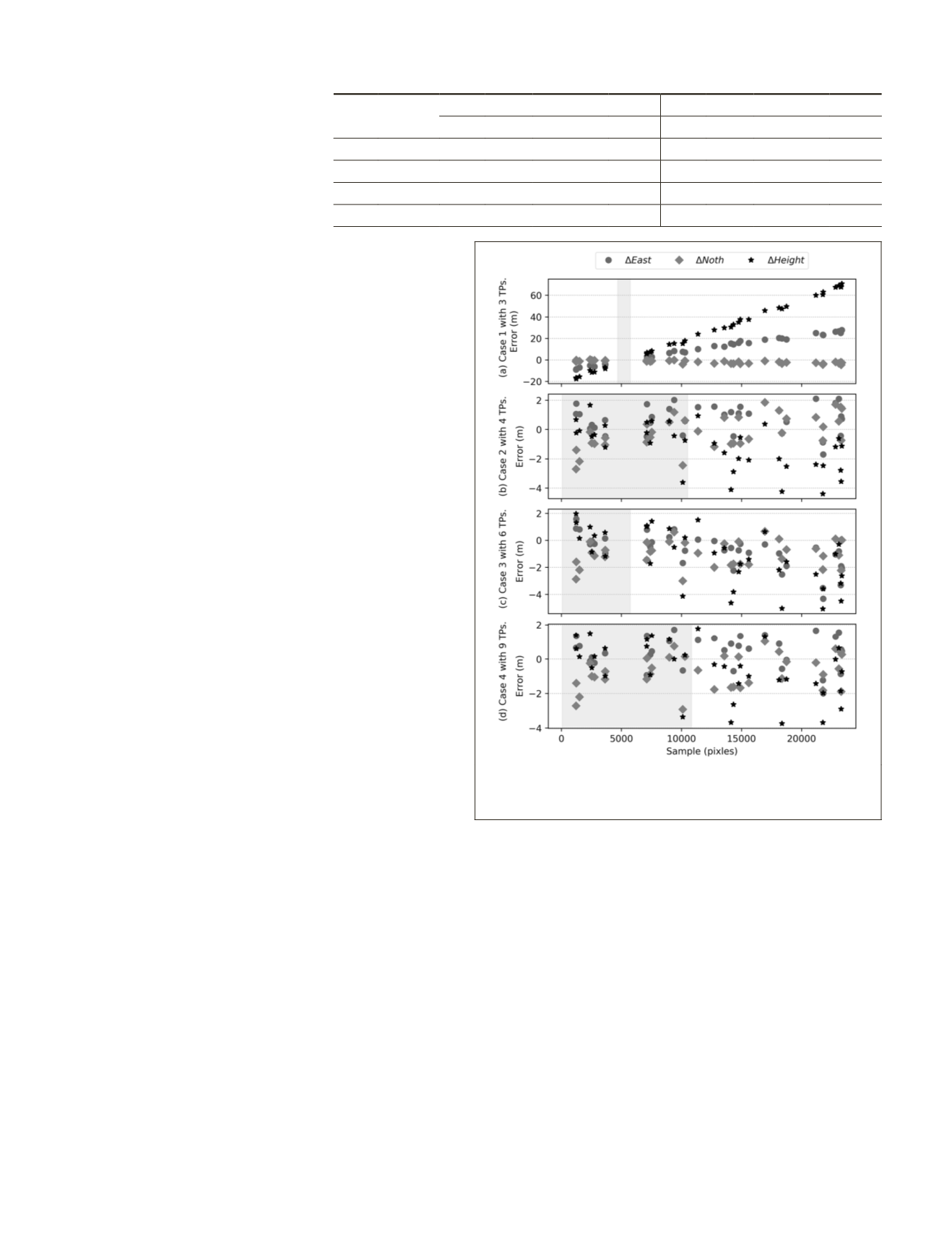
of Case 1 was 16.01 m
in planimetry and 27.79 m in height. The
maximum error of Case 1 was 27.91 m in
planimetry and 70.65 m in height. The
errors of the checkpoints in east, north,
and height were in linear correlation with the sample coordi-
nates, as shown in Figure 7a, which is consistent with Equa-
tion 12. In addition, the three-dimensional errors were close
to 0 at the tie point area, which corresponds to the shadow
area in Figure 7.
The
RMSE
was reduced to 1.66 m in planimetry and 1.99 m
in height when four tie points were used for Case 2. Compared
with Case 1, Case 2’s accuracy improved significantly. Figure
7b shows that the largest error, 2.90 m in planimetry and −4.40
m in height, occurred at the end of the sample. Furthermore,
the error outside the tie point area was larger than that inside
the tie point area, because the extrapolation was applied for
the outside area. It was similar to the small lateral overlap area
if all tie points were distributed in a small part of the common
area. As shown in Figure 7c, the errors grew with the sample
coordinates, especially in height. According to Equation 12,
a smaller lateral overlap means that the error grows faster,
which can be observed in Figure 7c. In such a case, the
RMSE
was approximately 2.03 m in planimetry and 2.36 m in height.
When nine tie points were used, both the
RMSE
errors in Case
4 were smaller than those in Case 2 and Case 3.
The least-squares estimation minimizes the quadratic form
v
T
Pv
of image observations, because pseudo-observations
are not applied. Therefore, the tie points’ object coordi-
nates of different strips, calculated by forward intersection
independently, should be approximately equal after block
adjustments. However, the random errors of the tie points
are propagated into the distant check points by the ratio of
sample coordinates to lateral overlap, which results in the
geolocation error of these checkpoints changing with the
sample coordinates. To achieve higher accuracy, more well-
distributed tie points with higher precision and larger lateral
overlap are preferred.
All four strips were involved in the block adjustment to
compare the affine compensation and drift compensation. In
practice, checkpoints are involved in block adjustments as
tie points. Therefore, no additional tie points were used. Five
sets of
GCPs
were applied, including sets with no
GCPs
, four
GCPs
in the corners of the entire block, four
GCPs
in the first
strip, ten
GCPs
, and 22
GCPs
.
Block adjustment without
GCPs
is an ill-posed problem.
In this experiment, truncated singular value decomposition
(
TSVD
) was applied to obtain a certain solution. The geoloca-
tion errors of the entire block are illustrated in Figure 8. After
block adjustment, the geolocation errors of affine compensa-
tion varied from strip to strip. The process of block adjust-
ment can be divided into two iterative steps: calculating the
object coordinate of tie points with estimated compensation
models and estimating compensation models with the object
coordinates of tie points until the residual errors in the image
space are minimum. Initially, the intrinsic errors of the
RFM
caused bias in the object coordinates of tie points. In addi-
tion, the tie points in the overlap had different geolocation
errors. Therefore, the sample-dependent parameters
e
2
,
e
5
were
adjusted, although the yaw angle errors were not significant.
As a result, the horizontal and height errors of the first strip
were reduced from west to east, and the rest of the strips had
smaller height errors and growing horizontal errors from west
to east. However, the geolocation errors of the drift compensa-
tion model were almost equal, as shown in Figure 8b, because
the residuals in the image space were consistent over the
image after block adjustment with drift compensation. The
horizontal errors pointed to the northeast approximately 15
m, whereas height errors were approximately 2 m.
As expected, there were significant geolocation errors in
the second and third strips, when four
GCPs
were deployed in
the corners of the entire block. The random errors of tie points
could have been magnified by the ratio of sample coordinates
to lateral overlap, even though the gauge was fixed. The
intrinsic errors of the
RFM
play a major role in geolocation
errors when the magnified random errors are larger than the
intrinsic errors. Therefore, the checkpoints around the
GCPs
had small geolocation errors, as shown in Figure 9a. In this
case, the
RMSE
of the entire block was 9.32 m in planimetry
and 1.67 m in height. In contrast, the
RMSE
of drift compen-
sation was 2.21 m in planimetry and 1.53 m in height after
block adjustment with the same
GCPs
. The geolocation errors
Table 2. Accuracy of block adjustment using affine compensation
ID
Number
of TPs
RMSE (m)
Max (m)
East North Horizontal Height East North Horizontal Height
Case 1 3 15.83 2.39 16.01 38.95 27.79 -4.62 27.91 70.65
Case 2 4
1.20 1.15
1.66
1.99 2.10 -2.71 2.90
-4.40
Case 3 6
1.52 1.35
2.03
2.36 -4.33 -3.00 4.48
-5.08
Case 4 9
0.98 1.23
1.58
1.68 -1.99 -2.91 2.99
-3.74
Figure 7. Geolocation of errors of Orbit 3642 in east, north,
and height (the shadow area indicates the distribution area
of the tie points).
796
December 2018
PHOTOGRAMMETRIC ENGINEERING & REMOTE SENSING


