where
p
ci
,
p
ri
are the weights of the image measurements in the
column and row, respectively, and
v
is the residual in the image
space. Then, the corresponding normal equation matrix
N
is
N
=
A
T
Q
–1
A
(7)
where
Q
is the covariance matrix of
c
,
r
.
N
is invertible if there
are more than three noncollinear
GCPs
for a single scene.
For
HRSIs
with along-track stereo images, the overlap is
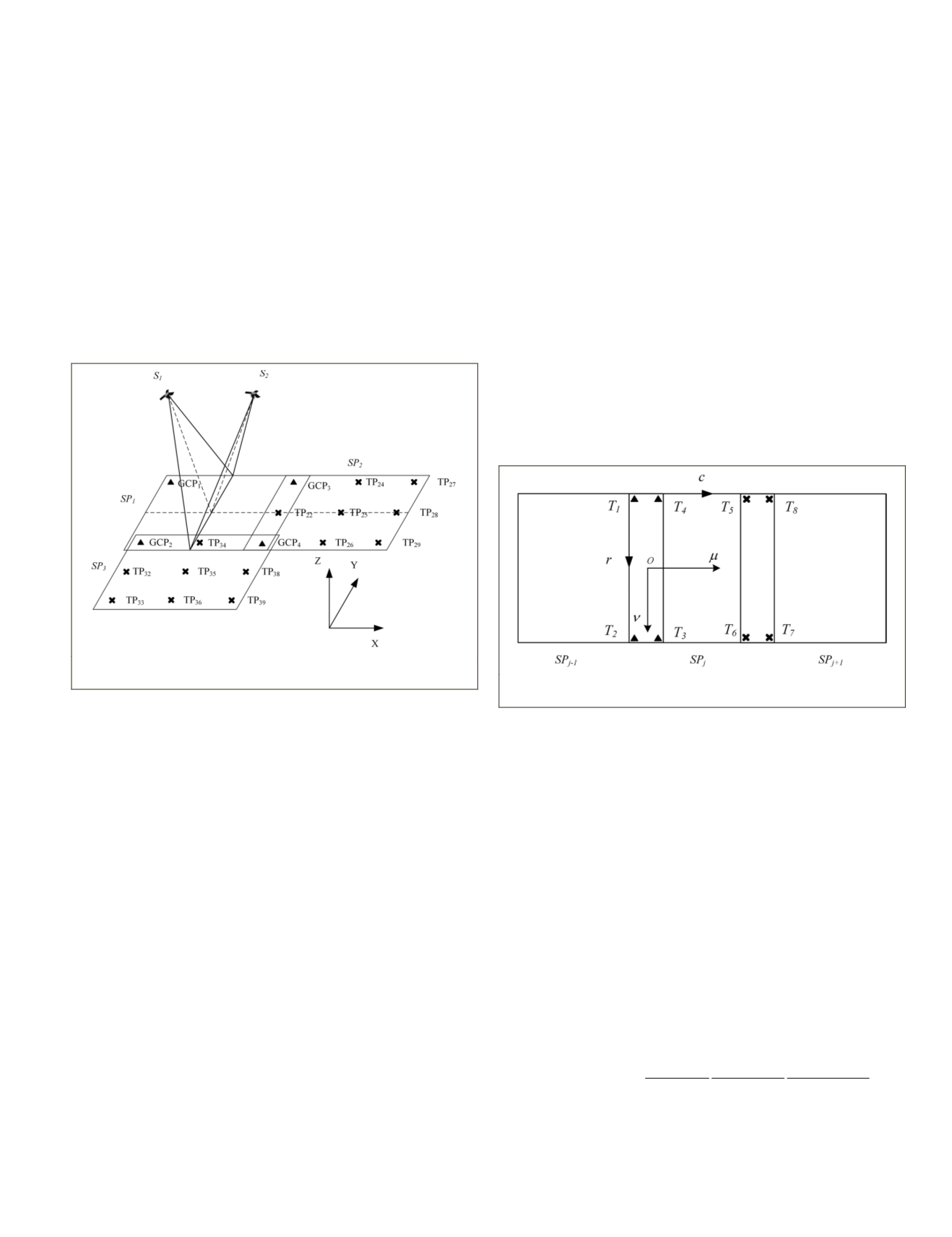
more than 90%. In this context, stereo pairs instead of single
scenes are used to analyze the precision of block adjustment.
As shown in Figure 1, the block area consists of three stereo
pairs
SP
1
,
SP
2
, and
SP
3
, in which
SP
1
and
SP
2
are from the
same strip, whereas
SP
1
and
SP
3
belong to two adjacent strips.
All four
GCPs
are deployed in the corners of the first stereo
pair
SP
1
, and there are 14 evenly distributed standard tie
points in the remaining stereo pairs.
Figure 1. Sketch map of the images and points for block
adjustment of the
HRSIs
.
The local object coordinates
XYZ
are established to esti-
mate the theoretical precision, with the
X
-axis along the strip
direction, the
Z
-axis vertical, and the
Y
-axis determined by
the right-hand rule. In such cases, the covariance of the two
elements
c
,
r
is 0. Then, the normal equation matrix shown in
Equation 7 is:
N
=
=
=
=
=
=
∑ ∑ ∑
∑ ∑
p
r p
c p
r p
r p
r c p
ci
i
n
i ci
i
n
i ci
i
n
i ci
i
n
i ci
i
n
i i ci
0
0
0
0
2
0
i
n
i ci
i
n
i i ci
i
n
i ci
i
n
ri
i
n
i ri
i
n
c p
r c p
c p
p
r p
=
=
=
=
=
=
∑
∑ ∑ ∑
∑ ∑
0
0
0
2
0
0
0
0
c p
r p
r p
r c p
c p
r c
i ri
i
n
i ri
i
n
i ri
i
n
i i ri
i
n
i ri
i
n
i
=
=
=
=
=
∑
∑ ∑ ∑
∑
0
0
2
0
0
0
0
i ri
i
n
i ri
i
n
p
c p
=
=
∑ ∑
0
2
0
. (8)
The reduced normal equation matrices
N
of
SP
3
are rank
deficient if seven tie points are deployed, as in Figure 1. The
object coordinate of
TP
34
is calculated with sufficient accuracy
when four
GCPs
are used for the orientation of
SP
1
using affine
compensation. However, equal sample coordinates of
GCP
2
,
GCP
4
, and
TP
34
result in the rank-deficient normal matrix
N
.
Therefore, a wider distribution of tie points (such as deploying
four tie points, one at each corner of the overlap area) is pre-
ferred. For the same reason, the adjacent scenes in the same
strip also suffer from ill-condition, and the same strip con-
straint is used to reduce the parameters (Zhang
et al.,
2014).
Theoretical Precision
The theoretical precision depends on many factors, includ-
ing the number and distribution of tie points and
GCPs
, the
imaging geometry, and the variance of observations. The
gauge is fixed by four
GCPs
in the first strip of the entire block,
and there are four tie points, one at each corner of overlap, to
achieve maximum distribution in the common area. Sub-
sequently, the precision of each strip could be determined
sequentially.
Let the width of the image be
w
, its height be
h
, and the
lateral overlap be
m
, as shown in Figure 2. The tie points of
the left strip
SP
j-1
are used as control points for the next strip
SP
j
, and
j
is the index of stereo sequences. Eight tie points,
distributed in each corner of the overlap, are deployed in
each stereo pair, while
T
1
,
T
2
,
T
3
, and
T
4
belong to
SP
j-1
and
SP
j
, whereas
T
5
,
T
6
,
T
7
, and
T
8
belong to
SP
j
and
SP
j+1
.
Figure 2. Error propagation between multiple strips in block
adjustment.
Because of the independence of
r
and
c
, their theoretical
precision is analyzed separately in the row and column direc-
tions. The variances in row
σ
r
2
and column
σ
c
2
of
T
1
–
T
4
consist
of two parts: variances of the object coordinates and variances
of the coordinate measurements. The weights of
r
and
c
are
p
r
=
q
r
–1
=
σ
0
2
/
σ
r
2
and
p
c
=
q
c
–1
=
σ
0
2
/
σ
c
2
, respectively, where
σ
0
is the
reference standard deviation, and
q
r
and
q
c
are cofactors of
r
and
c,
respectively.
First, the variance of a single stereo pair is elaborated. Let
the variance of the tie points
T
1
,T
2
and
T
3
,T
4
be
σ
1
2
=
σ
2
2
=
σ
0
2
/
p
1
and
σ
3
2
=
σ
4
2
=
σ
0
2
/
p
2
, respectively, where
p
1
is the weight of
T
1
,T
2
, and
p
2
is the weight of
T
3
,T
4
. For the sake of simplicity,
a local coordinate system
oμ
ν
is established, which moves the
origin of the image space to (
wm∙p
2
/(p
1
+p
2
), h/2
). In this co-
ordinate system, the image coordinates of
T
1
–T
4
are
(
-wm∙p
2
/
(
p
1
+p
2
)
, -h/2
)
,
(
-wm∙p
2
/
(
p
1
+p
2
)
, h/2
)
,
(
wm∙p
1
/
(
p
1
+p
2
)
, h/2
),
and
(
wm∙p
1
/
(
p
1
+p
2
)
, -h/2
)
,
respectively
.
Substituting the local
coordinates and weights of
T
1
–T
4
into Equation 8, the normal
equation matrix
N
is a diagonal matrix. The cofactor matrix of
the bias compensation parameters is
Q N
xx
= =
+
(
)
+
(
)
+
⋅
−
1
1 2
2
1 2
1 2
1 2
2 2
1
2
2
2
diag
p p h p p
p p
p p w m
. (9)
The variance of any point
T
i
, propagated from the bundle
adjustment parameters of the stereo pair
SP
j
, is
PHOTOGRAMMETRIC ENGINEERING & REMOTE SENSING
December 2018
793


