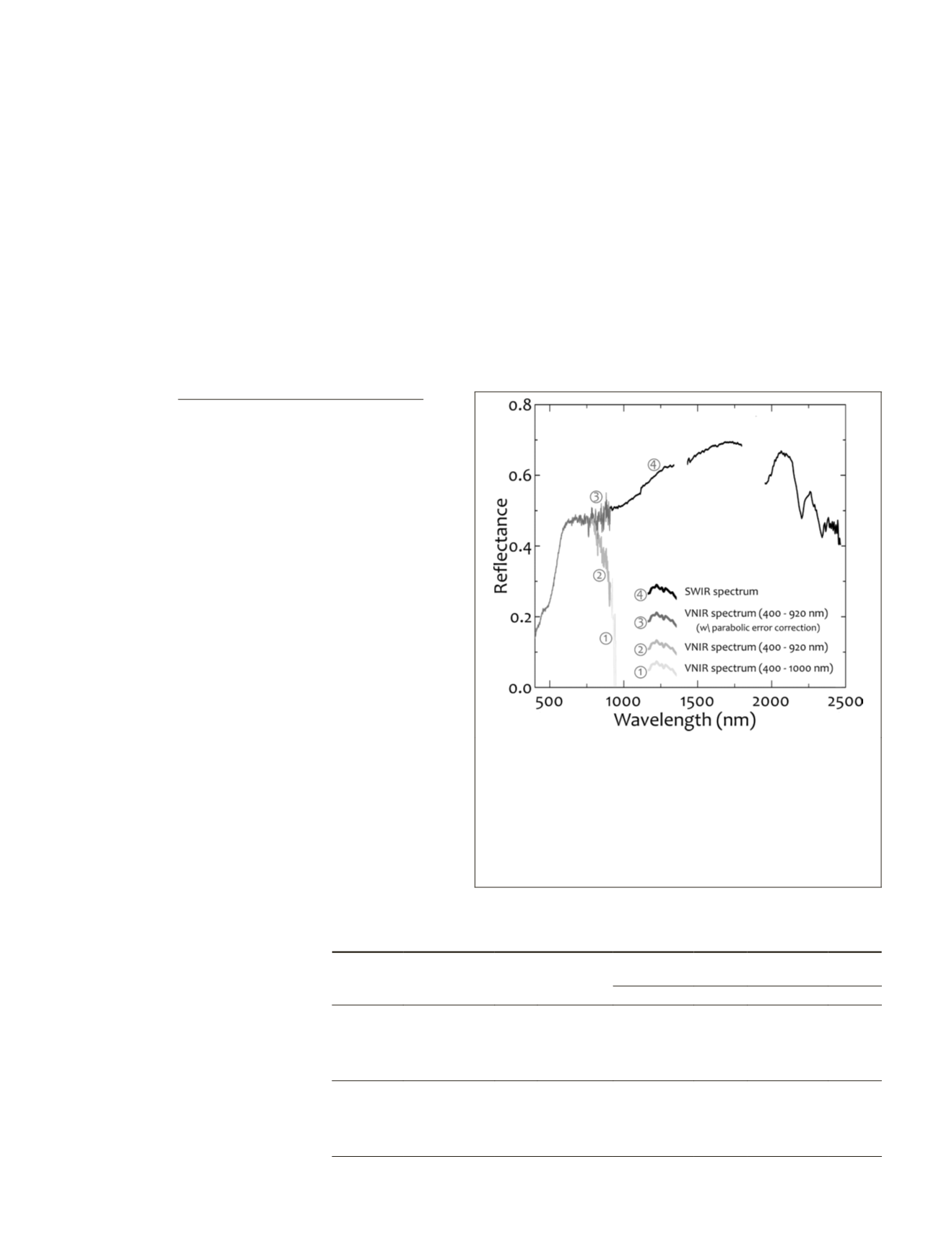
performance of the
VNIR
camera in wavelengths longer than
approximately 750 nm the reflectance profile plunges, which
appears to follow a parabola (Figure 2). Consequently, this
parabolic error results in an offset between the
VNIR
and
SWIR
image spectra. Such errors need to be characterized and cor-
rected in order to obtain continuous
VNIR
+
SWIR
spectra. Simi-
lar problems regarding the reflectance offset were observed
in Murphy
et al
. (2012); however, no correction routine was
implemented and/or suggested. The reflectance offset due to
the parabolic error is very similar to that observed between
different detectors of the
ASD
spectroradiometers, for which a
correction method is suggested (FieldSpec Pro User’s Guide,
2002; Hueni and Bialek, 2017). In an effort to compensate for
the reflectance offset between
VNIR
and
SWIR
image spectra,
a parabolic correction routine was adapted from Hueni and
Bialek (2017), giving the correction coefficients (corrCoeff) for
the region between 753 nm and 920 nm based on the reflec-
tance offset at 920 nm:
corrCoeff
swir
vnir
753 920
753 920
2
920
920
753
:
:
(
)
(
) . (
)
=
−
−
(
)
λ
φ
φ
φ
920
2
920 753
vnir
(
)
−
. (
)
+1
where
λ
is the wavelength and
φ
is the reflectance. The coef-
ficients were then applied to the correction region at the end
of the
VNIR
spectrum accounting for the reflectance offset
between
VNIR
and
SWIR
spectra (
in Figure 2), which in turn
allows obtaining a continuous
VNIR
+
SWIR
spectrum.
Spectral Analysis and Image Classification
The combined
VNIR
+
SWIR
image spectra of the prominent
lithologies in the studied outcrop were compared to the labora-
tory reflectance spectra of the collected rock samples. Although
it is not a complete evaluation, this comparison could provide
insight on the performance of the implemented image co-reg-
istration and spectral concatenation. Subsequently, hyperspec-
tral image classification was performed using a well-known
algorithm: Mixture-tuned Match Filtering (
MTMF
) (Boardman
and Kruse, 1994). The
MTMF
classifier performs a partial un-
mixing to find the abundances of user-defined end-members
maximizing the response of the end-member while suppressing
the response of the background. The
MTMF
classifier requires
isotropic, unit variance data and thus, only the spatially
coherent
MNF
components were used as input. Further details
on the
MTMF
classifier can be found in Boardman and Kruse
(2011 and 1994). End-member spectra can either be obtained
from existing spectral libraries, laboratory or field measure-
ments, or can equally be extracted directly from the hyper-
spectral images. In this study, the latter approach was used.
The end-member spectra were identified using a statistical
procedure: pixel purity index (
PPI
). Although this approach has
been used to identify the most spectrally
pure (extreme) pixels, the end-member
spectra identified herein are not necessar-
ily spectrally pure but rather spectrally
distinct. As it typically performs better on
data with normalized noise, prior to
PPI
a
Maximum Noise Fraction (
MNF
) transfor-
mation (Green
et al
. 1988) was applied to
the data and only the spatially coherent
components were used.
Results and Discussion
Spatial Image Co-registration
A brief summary of the
SIFT
runs is
given in Table 2. The first run of
SIFT
was performed using image bands at
similar wavelengths. Considering the size of the input im-
ages, the number of matching points is relatively low. This
could be attributed to relatively low sensitivity of the
VNIR
camera sensor at this wavelength resulting in speckles. The
subsequent runs were performed in an attempt to increase
the number of matching points. The second run used input
image bands with the highest signal-to-noise ratio calculated
over the ~30% calibration panel (Atkinson
et al
., 2005). For
the third run, the input images were obtained from principal
component analyses of the
VNIR
and
SWIR
bands within the
overlapping spectral range. The eigenvector loading signs and
eigenvalues indicated that the first principal component from
both analyses represents most of the information within the
data. Lastly, for the fourth run, the input images were ob-
tained from principal component analyses of the entire
VNIR
and
SWIR
spectra.
The overall quality and fitting error of geometric transfor-
mations were evaluated based on the root-mean-square error
(
RMSe
). In both transformation methods, using the points
Figure 2. A sample image spectrum before and after the
parabolic error correction.
VNIR
spectrum between 400
nm and 1000 nm. Due to the increasing noise towards the
end of the spectrum; wavelengths larger than 920 nm were
excluded from further processing.
VNIR
spectrum between
400 nm and 920 nm,
before and
after the parabolic
error correction applied for the region between 753 nm
and 920 nm.,
SWIR
spectrum, atmospheric absorption
wavelengths at around 1400 nm and 1900 nm are excluded.
Table 2. Summary of scale-invariant feature transform (
SIFT
) runs along with overall
RMSe
and highest individual point error of subsequent spatial co-registration of
VNIR
and
SWIR
images.
Image Size
Image
Bands
SIFT
runs
# of inliers
/ total
matches
Registration
RMSe (pixels)
Highest individual
point error (pixels)
polynomial affine polynomial affine
150 × 1064
(VNIR)
909.40 nm
1
st
211/231
0.8288 0.8478
3.44
3.46
909.17 nm
584.62 nm
2
nd
611/666
0.5651 0.5741
1.97
3.45
1283.22 nm
140 × 1040
(SWIR)
PC1 (VNIR)
3
rd
447/487
0.5159 0.5192
1.94
2.96
PC1 (SWIR)
PC1-2 (VNIR)
4
th
745/811
0.5884 0.6042
1.97
3.42
PC1-2 (SWIR)
784
December 2018
PHOTOGRAMMETRIC ENGINEERING & REMOTE SENSING


