Results
Models Results and Evaluation
In this paper, a significant correla-
tion between
ECa
and remotely
sensed data was considered for
developing models using the Partial
Least-Squares Regression (
PLSR
)
method. The variables (i.e.,
SAVI
Index, (Red Edge) B6, (Near-IR1) B7
and (Near-IR2) B8) were grouped in
different ways and four
PLSR
models
(Model-A, Model-B, Model-C , and
Model-D) were developed. Details
of each model are shown in Table 6.
As is displayed in the table, Model-
A (M-
A
) was based on
ECa
and an
individual variable (
SAVI
), and
showed the lowest determination
coefficient (
R
2
= 0.25). Model-B was
developed using
ECa
and two vari-
ables (
SAVI
, Band-6), and revealed
a higher determination coefficient
than model-A (
R
2
= 0.62). Model-C
used
ECa
and three variables (
SAVI
,
Band-6, Band-7), and indicated an
even higher determination coef-
ficient (
R
2
= 0.64). Model-D used
all variables (
SAVI
, Band-6, Band-7,
Band-8) and showed the highest
determination coefficient (
R
2
=
0.67). Overall, the order of deter-
mination coefficient values for all
models was M-
D
> M-
C
> M-
B
> M-
A
.
The
PLSR
model with four factors
(M-
D
) was selected based on the rule
that the addition of another factor
should reduce the
RMSE
by more
than 2 percent (Maimaitiyiming and
Ghulam, 2017; Chen and Gu., 2009;
Cho and Skidmore, 2007).
The scatter (plots between the
measured and predicted values) of
each model is displayed in Figure
4. In combination with the root
mean square errors (
RMSE
), model
M-
D
performs better with
RMSE
=
1.19 dS·m
-1
and model M-
A
fits
poorly with
RMSE
(1.83 dS·m
-1
).
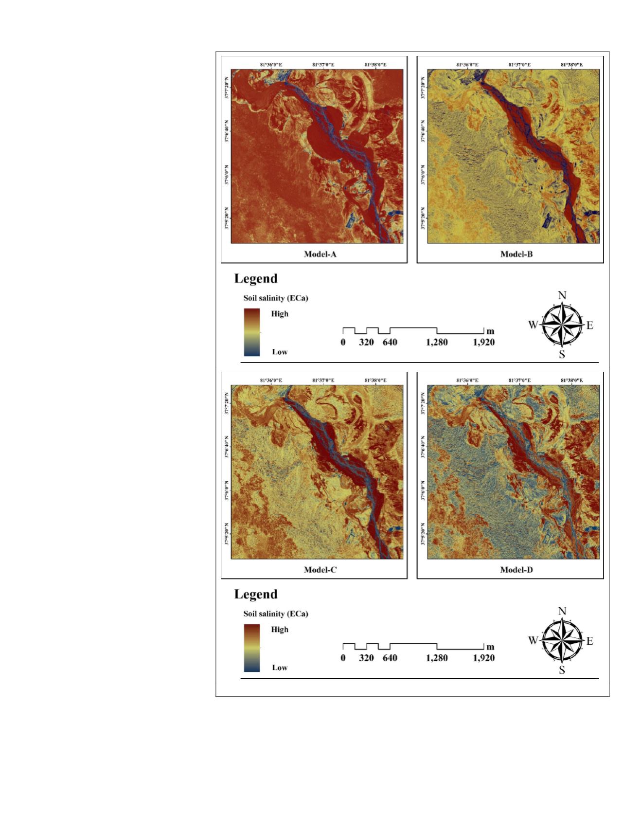
According to the four types of
PLSR
models, soil salinization inver-
sion maps were generated (Figure
5). From the spatial scale analysis,
model M-
A
has very poor ability to
identify ground objects, and it is dif-
ficult to distinguish between saline
and non-saline areas; model M-
D
is
more powerful in identifying saline
soil. On the basis of field investiga-
tion, the model M-
D
has the best
inversion capability in the study
area. Therefore, to compare the four
models, model M
-D
with
R
2
= 0.67,
RMSE
= 1.19 dS·m
-1
(
P
<0.01) indicated that the measured and
predicted values of soil conductivity were highly correlated
and had good potential for estimating and mapping soil salinity.
The final results showed that the integration of sensitive bands
[(Red Edge) B6, (Near-IR1) B7, (Near-IR2) B8] of soil salinity
(
ECa
) and soil adjusted vegetation index (
SAVI
) derived from
WorldView-2 data has good potential for predicting soil salinity.
Spatial Variation in Soil Salinity Maps
In this study, model M-
D
proved to be promising for mapping
soil salinity (
ECa
). According to the optimal
PLSR
model, the
spatial distribution map of soil apparent conductivity was
made using
ENVI
software. In accordance with the classifica-
tion rules of soil electrical conductivity (Shirokova
et al
.,
2000; Farifteh
et al
., 2010), the spatial classification map
was further categorized into four levels of soil salinity. These
Figure 5. Soil salinity map for the part of the Keriya Rive based on four
PLSR
models.
PHOTOGRAMMETRIC ENGINEERING & REMOTE SENSING
January 2018
49


