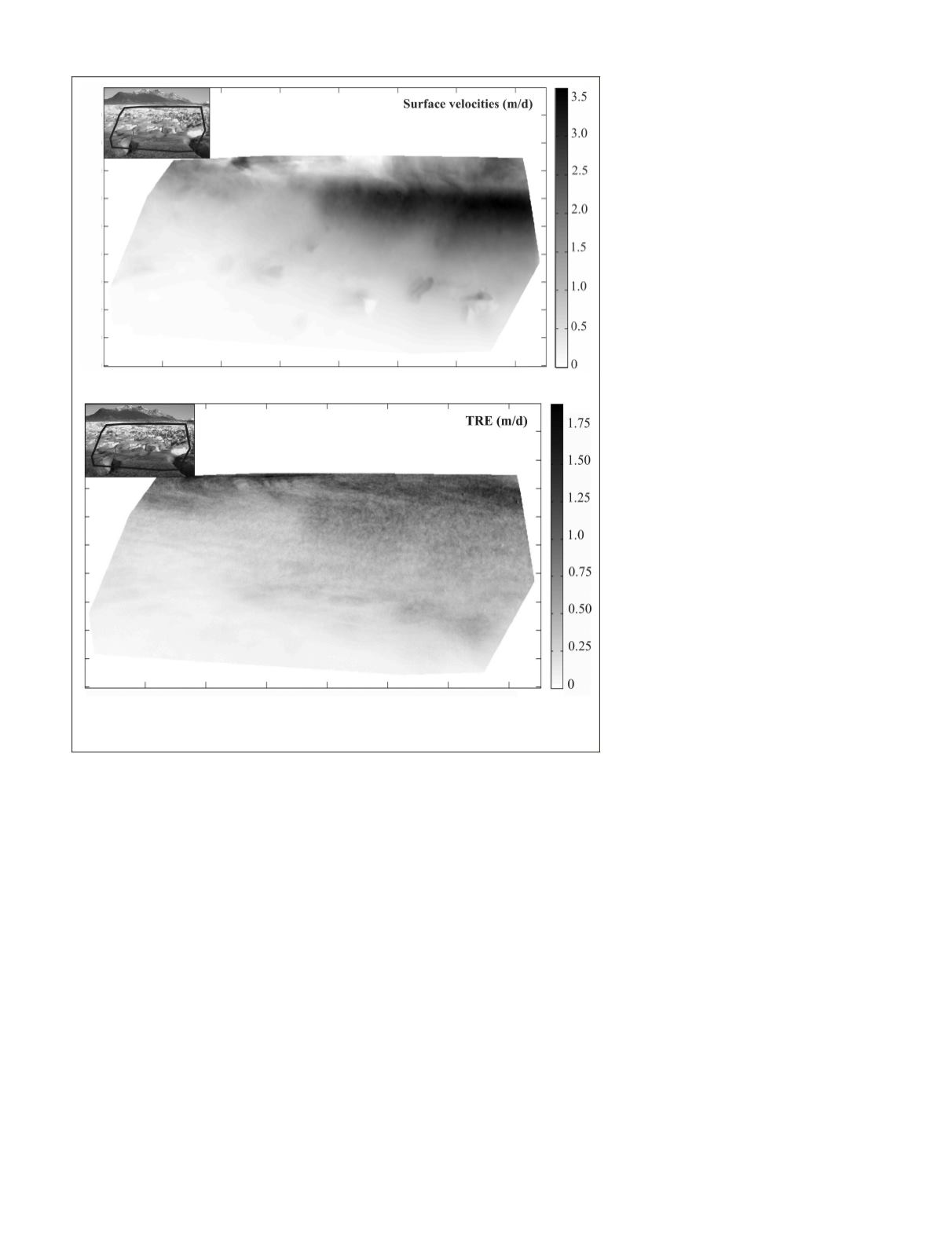
field is calculated from the average magnitudes of 231 image
pairs, and the mean surface velocities reach values between
3.5 m/d and 0.5 m/d (meters per day) in the central area and
near to the margins, respectively. The fast flow area is mainly
concentrated at the central part, pictured in black, while the
slow moving ice areas are mainly located toward the mar-
gins shown in light grey. This pattern is consistent with the
expected ice flow acceleration toward the glacier front central
part, and with the slow moving ice near the margins. This
near front acceleration has been previously described for other
calving glaciers in Patagonia (Sakakibara
et al
., 2014), where
calving is driven by deep water near the front. At the Viedma
glacier, this is confirmed by the recently surveyed bathymetry
of the lake, where up to 571 m water depths were detected.
Note that between April 2014 and March 2016, the central
part of the glacier front retreated near 800 m, as detected by
satellite images. Former results, obtained by offset tracking
Synthetic-Aperture Radar (
SAR
) imagery between April to
June 2012 by Riveros
et al
. (2013) showed values less than 4
m/d at the terminus area. Mouginot and Rignot (2015), using
radar and Landsat images between 1994 and 2014, provided
surface velocities in the range of 1 and 2 m/d near the end
part. Furthermore, we conducted surface velocities estimation
of Viedma glacier by LANDSAT images, acquired in October
and February 2015, and March 2016, using
the feature tracking technique (Lo Vecchio et
al., in review). These results at the termi-
nus show similar patterns obtained in the
present study, with an acceleration of the
front where maximum values reached 2.5
±0.3 m/d. Therefore, the different values of
velocities found in these investigations are
reasonably close to each other and can be
explained by different sensors and geospa-
tial data acquisition platforms, techniques,
creating different spatial and temporal reso-
lution data, plus the algorithms used.
Figure 5b shows the
TRE
axb
for the entire
study period, displaying a range from 1.8
m/d until 0.2 m/d. The largest errors are
reported for the area located at the glacier
surface and mountain border area. In this
zone, the computation of the optical flow
was less accurate due to the larger object
distance; note that the
TRE
axb
mean value
reached 0.36 m/d. In addition, based on
Equation 2, Figure 6 shows the mean error
(grey) for each image pair in the filtered time-
lapse sequence (231 pairs), and the standard
deviation (black) is shown as error bar only
for the large peaks. The average mean and
standard deviation are 5.7 ±7.9 in pixels (in
the image domain). This graph allows visual-
izing anomalous pairs used in optical flow
computation, despite passing the
CA
test. The
large peaks are closely related to big changes
in lightness between the images in an image
pair; in almost all cases, there was a presence
of clouds in some region, snow cover, and
not-uniform melting of the glacier surface,
as described by Vogel
et al
. (2012), which
affect the motion computation. The velocity
estimation can be further refined by applying
the constraint of slowly changing velocity;
an effect known from glacier dynamics. So
applying a low-pass filter and then removing
outliers can measurably bring down the stan-
dard deviation of the velocity estimation.
Figure 7a and 7b show the reconstructed
errors for two examples. The top frames show the images
that define the image pair for the
LDOF
computation. Figure
7a shows a case of changing lighting conditions, resulting in
significant errors in the computation of
LDOF
. Below the left
image, the results of the
LDOF
are shown with color-coding for
better visualization (Liu
et al
., 2011); clearly, very poor optical
flow computation performance. Each pixel symbolizes a vec-
tor where the magnitude and orientation are the function of
the tonality and saturation of the pixel value. Below the right
image, the error reconstruction is shown. Note that it is easy
to identify the cause of these errors because the objects, such
as presence of clouds, changes in snow cover, or shadows over
the crevasses, appear and disappear between the images pairs.
In contrast, Figure 7b shows an example with good lighting
conditions where the error remains low over the entire area.
Note the interesting situation in the middle of the frame, where
the presence of people is observed, clearly indicating the abil-
ity of the
LDOF
to detect small changes with high precision.
Conclusions
In this work, we have applied dense optical flow field method
to estimate glacier movement at high accuracy. The feasibility
(a)
(b)
Figure 5. (a) Flow vectors in meters per day (m/d), and (b) Error model based
on
TRE
assessment.
PHOTOGRAMMETRIC ENGINEERING & REMOTE SENSING
January 2018
39


