Data Analysis and Soil-Adjusted Vegetation Index (
SAVI
) Selection
Soil conductivity data (
ECa
) were obtained using an EM38-
MK2
meter, and measurements were taken at 361 points along 12
transects through the study area. Based on an analysis of the
original data, abnormal values that were caused by natural
factors were eliminated to reduce their influence on the accu-
racy of the model. To build the
PLSR
models, according to the
electrical conductivity values, the samples were sorted from
height to low using SPSS
®
(Version 19.0). Subsequently, the
data were divided into two subsets by uniformed-space. One
subset was used for training (
n
= 261), and the other subset
was used for testing purposes (
n
= 100). The main descriptive
statistics of electrical conductivity data are given in Table 3.
As can be seen in the table, the average values of
ECa
that cor-
respond to the calibration set and the validation set were 4.57
dS·m
-1
and 4.69 dS·m
-1
, and the coefficients of variation were
43.54 percent and 46.90 percent, respectively. An average
ECa
value from all sampling points in the study area was 4.60
dS·m
-1
, which is between the mean value both of calibration
and validation sets. The coefficient of variation (
CV
) was 44.57
percent, which is a medium variation degree, and the value
range was between the
CV
of the calibration set and the
CV
of
the validation set.
In all spectral indices, the soil adjusted vegetation index
(
SAVI
) was selected to evaluate soil salinity in the study area.
The index attempts to minimize brightness-related soil effects
by considering first-order soil vegetation interaction by means
of a soil-adjusted parameter (
L
is shown in Equation 1), which
usually depends on the vegetation coverage and has to be
empirically determined. However, it can also be measured.
In particular, for the case of intermediate vegetation canopy
levels, authors have suggested the value
L
= 0.5 (Huete, 1988;
Gilabert
et al
., 2002).
SAVI
= [(NIR – Red)/(NIR + Red +
L
) × (1 +
L
)
(1)
where Red is the red band, NIR is the near-infrared band of
the WorldView-2 image, and L is a soil adjustment factor.
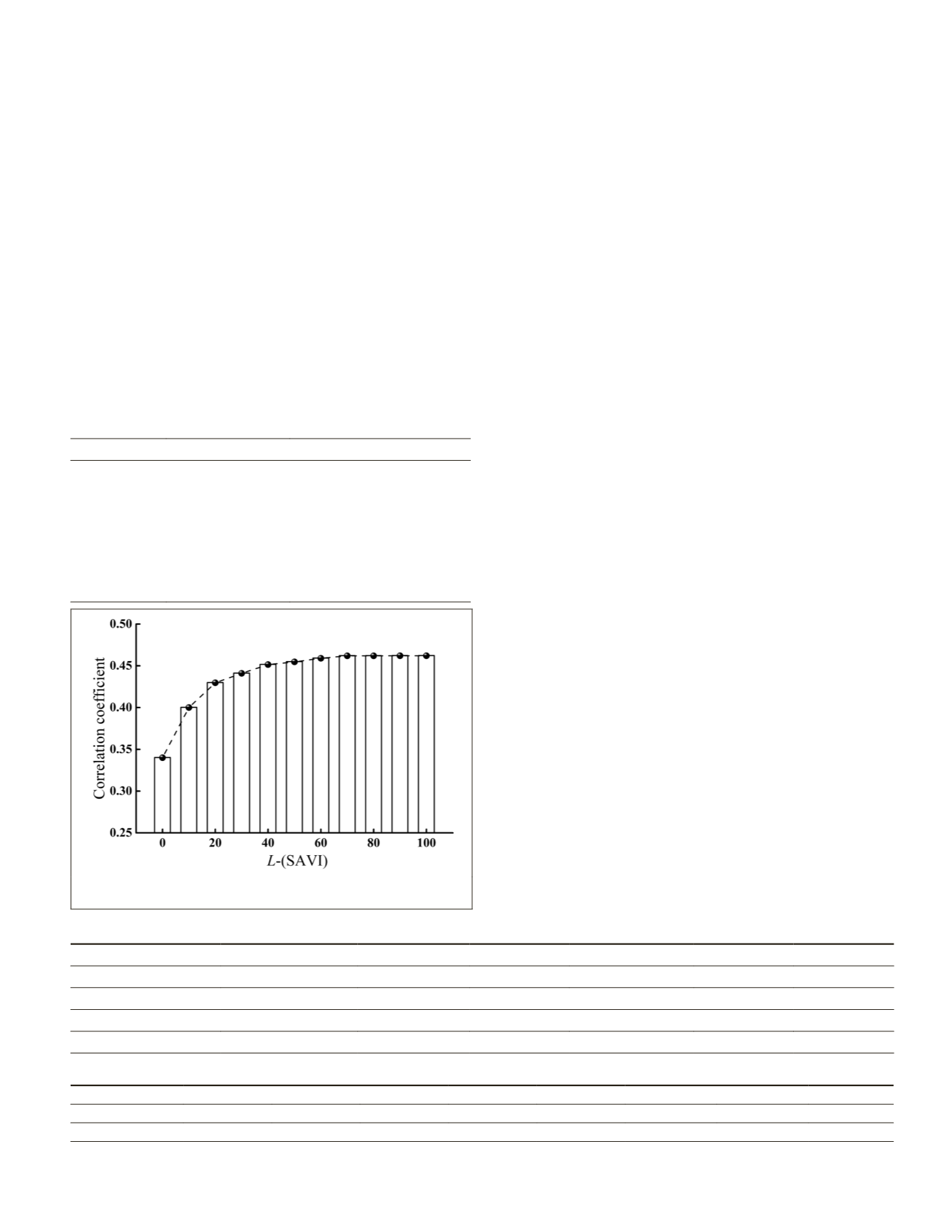
It was observed that as
L
changes the correlation between
the
SAVI
and
ECa
also changes, which is shown in Figure 3. As
depicted in the diagram, the range of parameter L varies from
0 to 100, and the correlation between
SAVI
and
ECa
gradually
improved. As the
L
value increases to 100, the correlation
maintains a steady trend. The highest correlation coefficient
corresponds to the
SAVI
index as a sensitivity index and was
selected as the modeling variable.
Following the correlation, a Pearson Correlation analy-
sis was conducted between
ECa
and Bands derived from the
Worldview-2 image. The reflectance of bands corresponding
to each sampling point were extracted using the
ENVI
(Version
5.1) software, and correlation analysis was performed based
on SPSS software. Detailed results are shown in Table 4. As
can be seen in the graph in Figure 4, the reflectance of bands
((Coastal) Band1, (Blue) Band2, (Red Edge) Band6, (Near-IR1)
Band7, and (Near-IR2) Band8) had a significant correlation (
P
<0.01) with the
ECa
data, whereas a low correlation appeared
between bands (Band4, Band5) and the
ECa
data. The best
correlations were obtained with bands ((Red Edge) Band6,
(Near-IR1) Band7, and (Near-IR2) Band8) and were selected as
sensitive bands and modeling variables.
Model Validation
Validation of the models is an important step to ensure
models quality (Karunaratne
et al
., 2014; Fidahussein,
et al
.,
2004), Once all the developed models were tested, models
with (a) A high
R
2
, indicating that a strong linear relationship,
(b) Low root mean square errors of the model’s variables. The
two quantitative criteria between measured and predicted
values were calculated by the equation listed in Table 5. As
a result, the best implemented
PLSR
model that met all the
model selection and validation criteria was picked and used
to predict and map the spatial variation in soil salinity.
Table 3. Statistical characteristics of the Apparent Electrical Conductivity (
ECa
) of sampling points.
Type of sample
Observations
Max (dS·m
-1
)
Min (dS·m
-1
)
Mean (dS·m
-1
)
SD (dS·m
-1
)
CV (%)
Whole set
361
9.95
0.30
4.60
2.05
44.57
Calibration set
261
9.88
0.30
4.57
1.99
43.54
Validation set
100
9.95
1.10
4.69
2.20
46.90
Max: maximum; Min: minimum; SD: standard deviation; CV: coefficient of variation
Table 4. Correlation coefficient between
ECa
and remotely sensed data.
Variables
Band1
Band2
Band3
Band4
Band5
Band6
Band7
Band8
ECa
0.29**
0.22**
0.12*
0.05
ns
0.03
ns
-0.43**
-0.55**
-0.57**
Significant:
*
P
<0.05;
**
P
<0.01; ns=not.
Table 2. WorldView-2 spectral details.
Bands
Wavelength (nm)
Resolution
Coastal
Blue
Green
Yellow
Red
Red Edge
Near-IR1
Near-IR2
Panchromatic
400-450
450-510
510-580
585-625
630-690
705-745
770-895
860-1040
450-800
Multispectral:
1.85 m
GSD
at nadir,
2.07 m
GSD
at 20° off-nadir
Panchromatic:
0.46 m
GSD
at nadir,
0.52 m
GSD
at 20° off-nadir
Figure 3. Correlation between
ECa
and
SAVI
index in
different soil adjustment factors.
PHOTOGRAMMETRIC ENGINEERING & REMOTE SENSING
January 2018
47


