and Förstner, 2005) fits best for the Ladybug5 camera heads.
Therefore, we assumed the equidistant projection model for
all individual heads of both Ladybug5 panorama cameras (II
& III). We estimated the same
IOP
set with two radial and two
tangential distortion parameters for both projection models
(perspective and equidistant). Moreover, we defined the left
cameras of each stereo system as origin of the ROP.
In a second step, we estimated part two of
BA
between the
navigation center and camera I.1 in our outdoor calibration
field. The parameters were estimated using bundle adjustment
incorporating the previously determined
IOP
and ROP. Finally,
we computed
BA
parameters for each stereo system with both
BA
parts (see Figure 9).
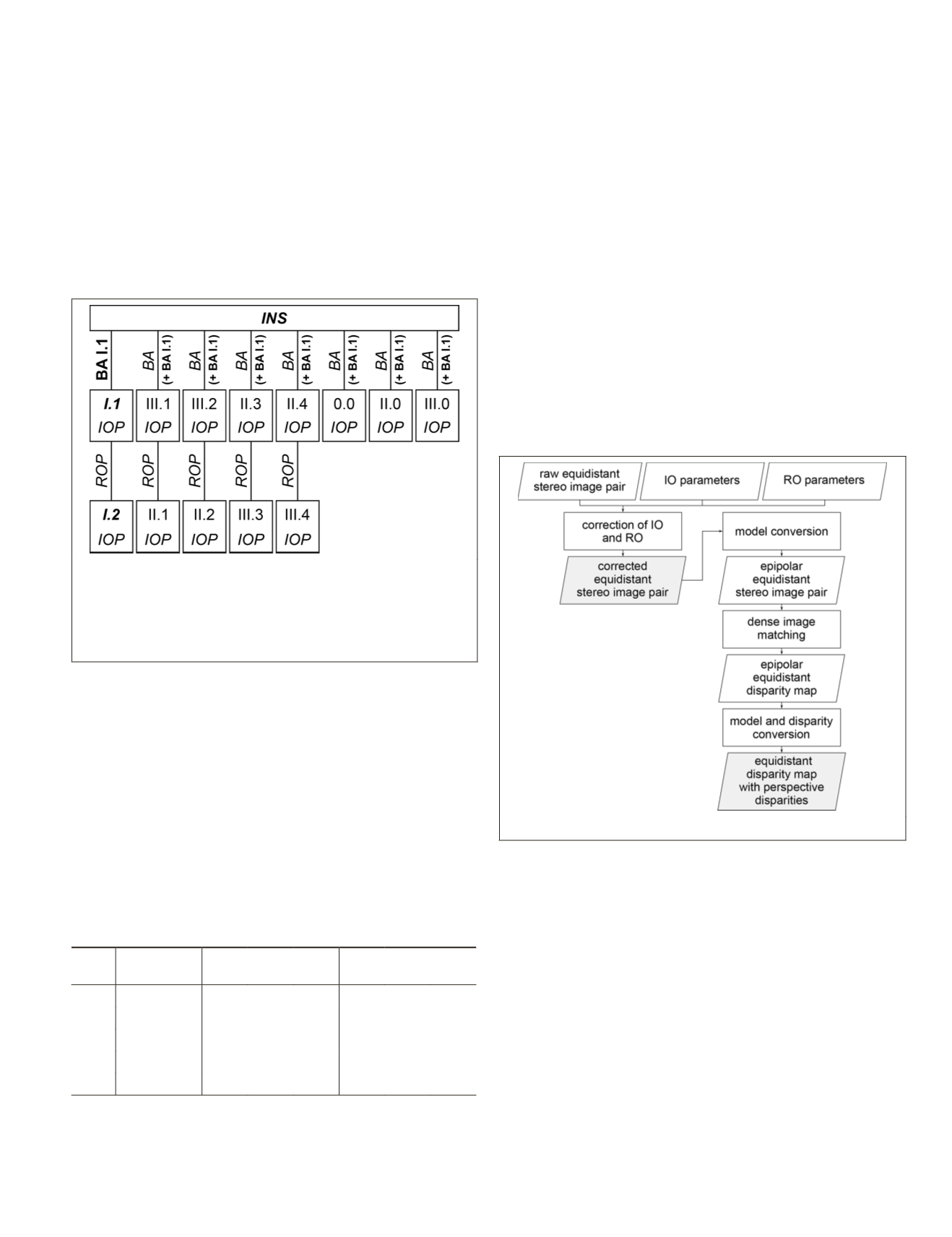
Figure 9. Functional model of the constrained bundle adjust-
ment (II) for outdoor calibration. We estimated the bold
parameter, fixed the italic parameters, introduced image
observations of the bold italic camera heads, and
INS
observa-
tions into the computation. Subsequently, we offset the
BA
parameters with the bold (
BA
I.1.) parameter in brackets.
The calibration results listed in Table 3 give an indication
of the achievable calibration accuracy. Since all estimated
parameters are highly correlated, their separate analysis is not
appropriate. The accuracy of target point definition, the image
measurement accuracy, the measuring arrangement, and the
suitability of the
IO
model influence the ROP calibration accu-
racy. The error from the navigation system additionally affects
the accuracy of the
BA
. Table 3 shows that the individual Lady-
bug5 heads (II & III) can be calibrated with the same precision
as the front pinhole cameras (I & 0.0). However, due to the large
opening angles of the cameras II & III, the orientation uncer-
tainty of the calibration can theoretically affect the variances of
the distance component from 1 cm up to 8 cm at a measuring
distance of about 10 m depending on the image region.
Table 3. Precisions of the calibration of relative orientation
(
RO
) as well as boresight alignment (
BA
) parameters.
Cam
Calibration
parameters
Std. dev. of
Position [mm]
Std. dev. of
Orientation [mdeg]
X Y Z
ω φ
κ
0.0
RO
0.3 0.3 0.5 10.0 20.0 2.0
II & III
RO
0.1 0.1 0.2 10.0 7.0 2.0
I
RO
0.1 0.1 0.3 13.0 24.0 3.0
I
BA
11.7 5.5 6.2 12.0 22.0 6.0
Processing Workflow
Our processing workflow aims at obtaining metric Geospa-
tial 3D Images for cloud-based 3D geoinformation services,
e.g., for infrastructure management or urban planning. As
suggested by Nebiker
et al
. (2015), a geospatial 3D image
consists of a georeferenced and distortion corrected image
with spectral bands as well as additional channels supporting
depth and quality information, ideally for each pixel. As part
of this work, we focus on depth map generation. Ideally, the
depth component of 3D images is derived from stereo imagery
using dense image matching - in this case from raw equidis-
tant fisheye stereo image pairs - in order to obtain very dense
depth representations and to ensure the spatial and temporal
coherence of radiometric and depth data.
Our implemented image processing workflow is a light-
weight, straightforward, as well as easily scalable approach for
obtaining both corrected equidistant RGB images and equidis-
tant disparity maps with perspective disparities (see Figure 10).
The main reason for keeping fisheye images in the equidistant
model is to prevent data loss. We assume a model conversion
from equidistant to perspective on the client or at the applica-
tion level. The advantage of a disparity map in comparison
with a depth map is the higher resolution at short distances.
Figure 10. Workflow for fisheye image processing.
After image conversion to the perspective model, 3D
points can be determined either by 3D monoplotting based on
disparity maps (Burkhard
et al
., 2012) or by point measure-
ments in both images of a stereo pair.
Figure 10 illustrates our stereo fisheye processing work-
flow. First, we correct interior orientation (
IO
) and relative
orientation (
RO
) which results in a distortion free equidistant
stereo image pair with the same focal lengths and corrected
principal points. Parallel epipolar lines are required for stereo
image matching algorithms such as semi-global matching
(
SGM
) (Hirschmüller, 2008) or
tSGM
(Rothermel
et al
., 2012).
Therefore, a previous image model conversion from equi-
distant to epipolar equidistant is essential (Abraham and
Förstner, 2005). After dense image matching, we reconvert
both the geometric image model from the epipolar equidistant
projection model to the equidistant projection model and
disparities from the epipolar equidistant projection model
to the perspective projection model. Abraham and Förstner
(2005) provide the formulas for projection model conversion.
PHOTOGRAMMETRIC ENGINEERING & REMOTE SENSING
June 2018
351


