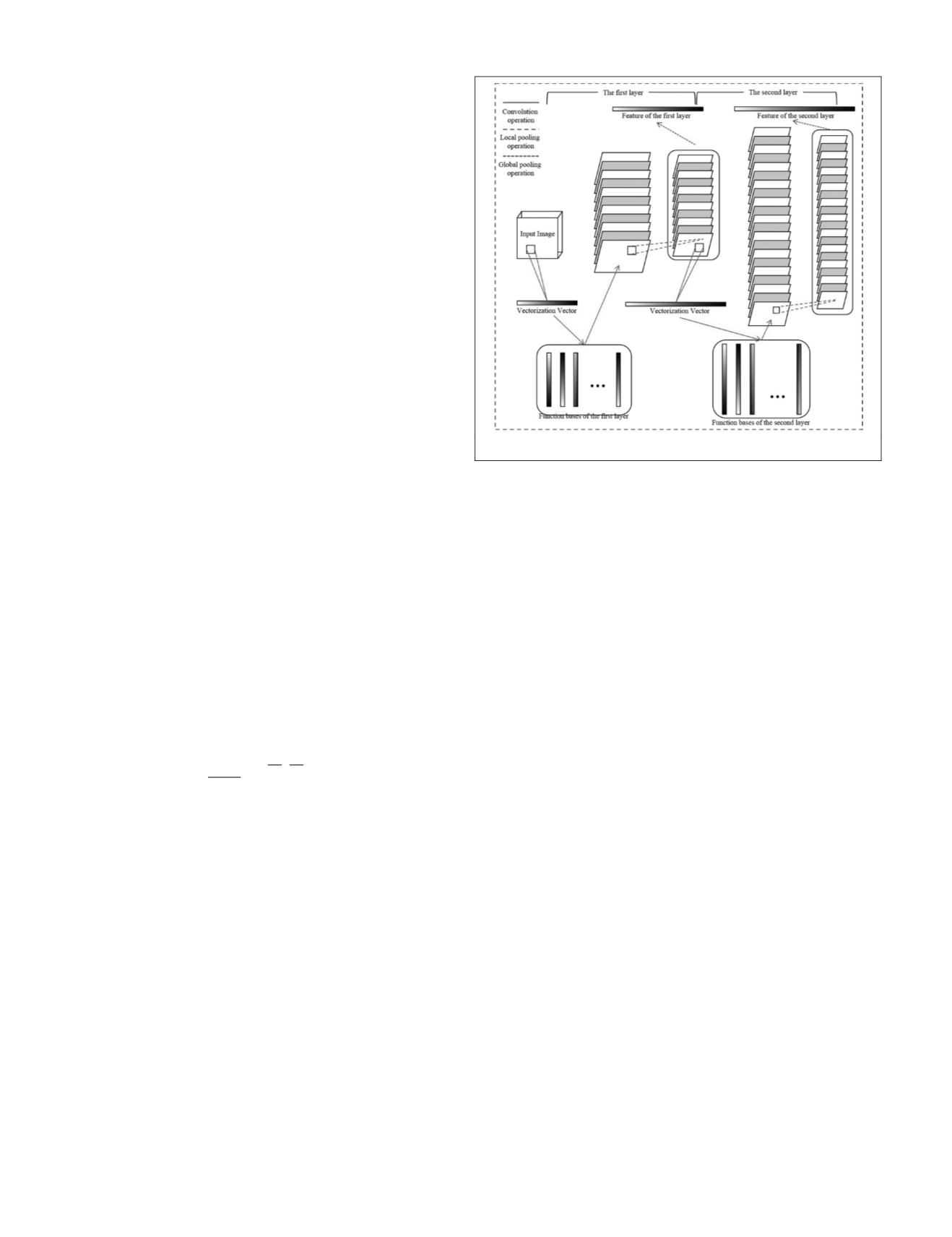
is divided into four quarters, and the averaging operation
is employed for each quarter. We let
g
1
,
g
2
,
g
3
,
g
4
denote the
corresponding feature vectors of every quarter, and then
the global pooling result can be expressed as G = {
g
1
,
g
2
,
g
3
,
g
4
}, where the dimension of G is 4 *
K
.
The multi-layer features can be obtained by repeating the
convolution, local pooling, and global pooling operations.
Specifically, taking the original image as the input of the first
layer and implementing the three operations, we can obtain
the feature extracted by the first layer, i.e., the result of the
global pooling operation. Then, taking the result of the local
pooling operation in the first layer as the input of the second
layer, we can obtain the feature of the second layer by the
three operations. The features of the higher layers can be
similarly extracted. Finally, we integrate the features of each
layer as the final multi-layer features.
The Proposed Tea Garden Scene Detection Framework
The proposed scene-based framework for tea garden detection
is illustrated in Figure 5. First, the whole remotely sensed
image is divided into a series of scenes, with each scene refer-
ring to an image block with a certain semantic category. Since
a tea garden does not always occupy all of a scene, we utilize
the overlapping regions to decrease the omissions, and the
size of an overlapping region is half of the scene. Then, based
on the extracted spectral and textural features, the
BOVW
,
sLDA
, and
UCNN
representations of each scene are computed,
respectively. Note that the dictionary in
BOVW
or the
UCNN
is trained by unlabeled data before detection. Finally,
SVM
,
which is an efficient classifier for remotely sensed image
classification (Huang and Zhang, 2013; Qin, 2015), is trained
using a small number of labeled samples to classify these
representations into tea gardens and non-tea gardens, expect
for the
sLDA
model, which can directly predict the category
of each scene after training. In addition, for the purpose of
a comparison, the scenes with spectral and spectral-textural
features are also directly classified with
SVM
.
In our work, the Gabor filter (Lee, 1996) is used to extract
the textural features due to its high efficacy in remote sensing
image texture description (Reis and Ta
ş
demir, 2011; Wang
et
al.
, 2014). It is defined as:
G
x y
ab
e
e
x
a
y
b i ux vy
,
(
)
(
)
(
)
=
− +
+
1
2
2
2
2
2
π
π
(3)
where
a
,
b
denote the scale along
x
and
y
, respectively, and
u
,
v
are the spatial frequencies of the filter in the frequency do-
main. To improve the calculation efficiency, the first principal
component acquired by principal component analysis (PCA)
is employed to extract the Gabor textures. In addition, for the
sample patches in the
BOVW
model, we calculate the mean
and standard deviation of each spectral/Gabor band as the
spectral/textural feature. In the same way, we also generate
the spectral and textural feature vectors for direct classifica-
tion with
SVM
, as a benchmark.
Experimental Data and Setup
Datasets
The experiments were carried out on four datasets, includ-
ing one remotely sensed image from the WorldView-2 (WV-2)
satellite and three images from Google Earth
®
. The details of
the four datasets are listed in Table 1, and the
RGB
images are
shown in Figure 6 (a). Dataset 1 was acquired from WV-2,
having eight spectral bands of a 2-m spatial resolution. Datas-
et 1 and dataset 2 were obtained at Longyan, Fujian province,
where the tea that is cultivated is mainly Oolong tea. The
tea in dataset 3 is Longjing tea, which is a famous green tea
mainly planted in Hangzhou, Zhejiang province. The area of
dataset 4 is Puer, Yunnan province, which is famous for the
cultivation of Puer tea.
Experimental Setup
The aforementioned datasets with different varieties of tea
were used to test the performance of the proposed scene-
based framework. For each testing image, 10 sets of samples
were randomly chosen, with each one containing 20 tea
garden scenes and 20 non-tea garden scenes as training data
to train the linear
SVM
and
sLDA
, and 200 tea garden scenes
and 400 non-tea garden scenes (independent of the training
scenes) as test data to assess the classification accuracy. In the
experiments, we selected the scenes with more than 90% of
the area occupied by tea garden as tea garden scenes, and the
scenes with no tea garden as non-tea garden scenes according
to Huang
et al.
(2015). The scenes with less than 90% of the
tea garden area were not considered in accuracy assessment.
In addition, Kappa was used as the evaluation criteria, con-
sidering the unbalanced numbers of tea garden and non-tea
garden scenes in the test data.
The parameters used in the four datasets are provided below:
1. Scene size: the size of each scene was 60 m × 60 m, i.e.
30 × 30 pixels for WV-2 imagery and 120 × 120 pixels for
Google Earth imagery. The sensitivity of this parameter is
discussed in the next section.
2. Spectral bands: 8 multispectral bands for WV-2 and 3
bands (red, green, and blue) for Google Earth images were
employed to generate spectral and textural features.
3. Gabor filter: The spatial frequencies
u
,
v
are expressed in
polar coordinates with radial frequency
f
and orientation
θ
. The parameters of the Gabor filter were set to
a
=
b
= 4,
f
= {0.006, 0.02, 0.06}, and
θ
= {0,
π
/3, 2
π
/3,}.
4. Topic model: For the
BOVW
model, the size of the learned
dictionary in each dataset (i.e., the number of cluster
centers of
k
-means) was set to 100. The parameters of
sLDA
were determined using 5-fold cross-validation.
5. Unsupervised feature learning: In our implementation, the
UCNN
trained by each dataset contained two layers, with
K
1
= 100 and
K
2
= 300, where
K
1
,
K
2
are the numbers of
Figure 4. Framework of unsupervised feature learning.
726
November 2018
PHOTOGRAMMETRIC ENGINEERING & REMOTE SENSING


