where,
P
a
= Coordinate of the captured point in the a-frame,
P
b
a
=
IMU
position in the a-frame (Note that this accounts for
level-arm offset between
IMU
and GPS sensor)
R
n
a
= Rotation matrix defined between local navigation frame
(n-frame) and a-frame;
R
n
a
=
−
( )
−
( )
∗
( )
( )
∗
( )
( )
−
( )
sin
sin cos
cos
cos
cos
sin
λ
φ
λ
φ
λ
λ
φ
i
i
i
i
i
i
i
∗
( )
( )
∗
( )
( )
( )
sin cos
sin
cos
sin
λ
φ
λ
φ
φ
i
i
i
i
i
0
(2)
λ
i
,
ϕ
i
are geodetic coordinates of
P
a
R
n
b
= Rotation matrix from body frame to local navigation
frame,
R
L
b
= Rotation matrix from lidar sensor frame to
IMU
(b-frame);
boresight rotation matrix
p
k
= Coordinate of the point in lidar sensor frame (as recorded
by the sensor)
Δ
T
L
b
= Offset between lidar sensor frame and the
IMU
boresight
translation.
The direct georeferencing Equation 1 indicates that at least
three sets of transformations are required to convert a feature
point measured by the lidar sensor in
SBF
to a global coordi-
nate system. One of the transformation is to determine the
boresight misalignment (rotation and translation) between
lidar frame and
IMU
body frame, denoted as
R
L
b
and
Δ
T
L
b
. The
focus of this paper is to develop innovative boresight calibra-
tion procedure to determine
R
L
b
and
Δ
T
L
b
for low density lidar
sensor based
MMS
. There are different methods available in the
literature to determine the boresight misalignment between
lidar sensors and
IMU
. The most common method used in com-
mercial grade mobile mapping systems is laboratory calibra-
tion (Habib et al., 2010). The laboratory method determines
the alignment of lidar sensor with respect to
IMU
in the factory
using precise calibration techniques. These values typically
remain unchanged unless the equipment is modified. In the
case of customized, in-house built mobile mapping systems,
modification of sensor alignment is inevitable due to the lim-
ited field of view provided by low-cost and low-density lidar
mobile mapping systems as previously described. Hence, a
method that can be used to calibrate at the user level is desir-
able. Additionally, in these systems, it is less likely that the
sensors will be strongly bolted and aligned to each other on
the platform. Thus, frequent computation of boresight mis-
alignment may become necessary for any reasonable mapping
applications.
Literature Review
Traditional calibration procedures use control points to deter-
mine the boresight misalignment. Considering the limitations
of identifying control points from low density scans, the re-
searchers have used higher level control features such as lines,
planes or free-form surfaces that are common between the
lidar point clouds that need to be calibrated or registered. The
concept of using control lines in 3D registration is discussed
in Jaw and Chuang (2008) and Nagarajan and Schenk (2016).
There are methods that use point-to-plane (Grant
et al
., 2012;
Schenk, 1999) and plane-to-plane (Acka, 2007; Bosché, 2012;
Dold and Brenner, 2006), where well-defined control plane
datasets are used in registration. Despite using line, plane or
surface features, most of these techniques use a point corre-
spondence instead of using complete features in the registra-
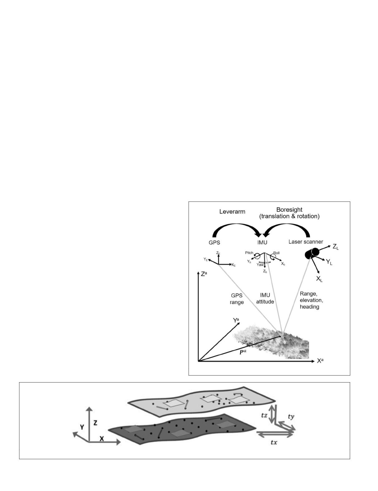
tion mathematical model. Figure 2 illustrates the concept of
registering 3D surface using points, lines, and planes. The
arbitrary surface (light gray) can be registered to control surface
(dark gray) to recover the transformation parameters
t
x
,
t
y
and
t
z
.
There are various in-flight boresight calibration methods
available in the literature. They typically look for a calibra-
tion field in the scene in the form of known control points,
lines, planes, or surfaces (Glennie, 2007; Siying
et al
., 2012;
Skaloud and Lichti, 2006; Skaloud and Schaer, 2007). Other
methods use multiple lidar scan lines in the opposite direc-
tions of a plane or sloped plane and over a building corner
to determine boresight angles (Rieger
et al
., 2010). These in-
flight methods are typically time-consuming and not practi-
cal for repeated calibration (Habib
et al
., 2010). In addition,
Figure 1. Mounting of different sensors in
MMS
.
Figure 2. Illustration of registration by using control points, lines, or planes.
620
October 2018
PHOTOGRAMMETRIC ENGINEERING & REMOTE SENSING


