these methods are mainly suitable for airborne lidar mapping,
where there are more features of interest available for match-
ing between the strips. Also, such systems typically use high-
precision
IMU
and lidar sensors that allow integrating error
models to better recover the boresight parameters.
Habib
et al
(2010) categorize boresight calibration ap-
proaches into system-driven and data-driven approaches.
System-driven approaches use mounting parameters and er-
rors in the lidar direct-georeferencing Equation 1 and deter-
mine them mathematically using control points. The errors
that can be incorporated into direct-georeferencing equation
are
GNSS
positioning errors,
IMU
attitude errors, lidar sensor
errors, etc., (Glennie and Lichti, 2010; Siying
et al
., 2012;
Skaloud and Schaer, 2007). Data-driven approaches use an
arbitrary 3D transformation between control data and lidar
point cloud (Le-Scouarnec
et al
., 2013). The major limitation
with the data-driven approach is that there is no one-to-one
relationship between individual systematic errors and the
transformation parameters. However, certain errors can be
eliminated if operated locally in a controlled environment,
(i.e., indoor in static mode) to generate the direct relation-
ship between the parameters and errors. The other systematic
errors in lidar such as horizontal and vertical rotation error,
horizontal and vertical offset and distance offset (Glennie and
Lichti, 2010) are assumed non-existent in effort to determine
only the mounting bias (boresight translations and rotations)
of lidar system with respect to
IMU
body frame. However, both
system-driven and data-driven approaches typically require
control points. Such methods require conjugate points to be
identified in both control and lidar point cloud data so that
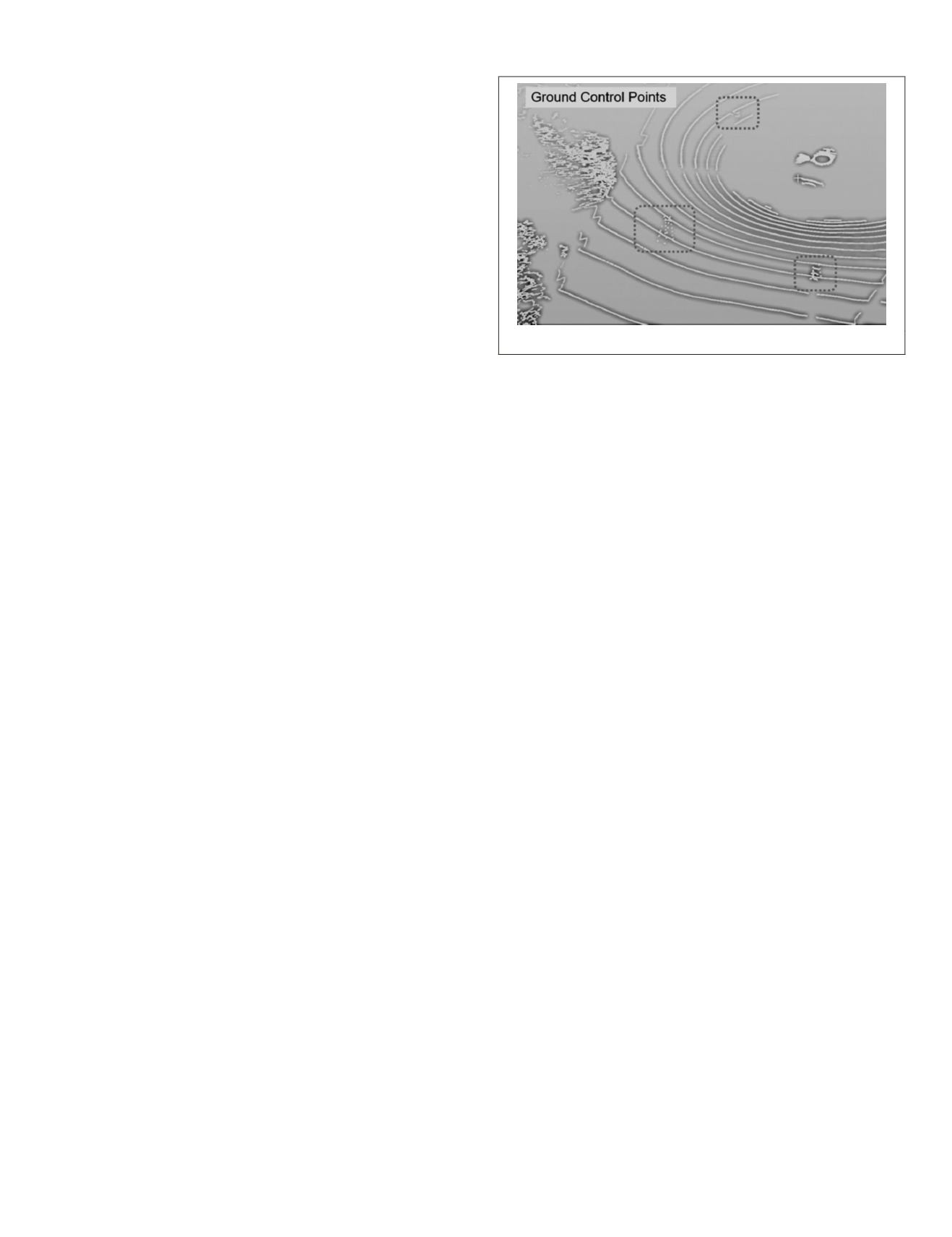
unknown boresight parameters can be determined Figure 3
shows a sample point cloud of a calibration field with three
GCPs
marked. As can be seen from this figure, identifying the
accurate location of the
GCPs
is nearly impossible. Hence, sev-
eral methods have been developed to use point-to-plane cor-
respondences for boresight calibration (Friess, 2006; Glennie,
2012; Glennie and Lichti, 2010; Skaloud and Lichti, 2006).
Some of the methods use natural surfaces instead of planes,
but still require point-to-surface correspondence (Filin, 2001;
Scaramuzza
et al
., 2007). Though identifying point-to-plane
is comparatively easier than point-to-point correspondence,
the wrong selection of points on corresponding planes can
result in completely different transformation parameters. This
research demonstrates a data-driven approach-based plane-to-
plane registration which is more comprehensive than point-
to-plane correspondence in determining unknown boresight
calibration parameters.
Methodology
This research demonstrates a method that takes all points
that constitutes conjugate planes into the registration math-
ematical model in contrast to just few sampled points. The
proposed data-driven calibration method assumes that only
mounting parameters that constitute 3D rotation (boresight
angles) and 3D translation (boresight translation) exist
between raw and registered point cloud. Hence, one-to-one
correspondence between mounting bias parameters and deter-
mined rigid body transformation parameters can be consid-
ered identical, as expressed in Equation 3:
X
′
=
R
(
α
,
β
,
γ
)
X
+
T
+
e
(3)
where,
X
′
vector consists of coordinates of points in the con-
trol plane; R is the 3D rotation matrix formed with the bore-
sight rotation angles (
α
,
β
,
γ
);
T
is the boresight translation;
X
– is the vector that contains coordinates of points on the
lidar plane, and
e
refers to random errors. This assumption of
eliminating other systematic errors is justified as the proposed
boresight calibration is performed in a laboratory without
using
GPS/IMU
data and by keeping the
MMS
static for the dura-
tion of the calibration process.
In the control-plane approach, the boresight calibration
method will determine the alignment between
IMU
and lidar
frame by minimizing the volume formed between low point
density lidar surface that is in
SBF
with unknown boresight
parameters and the control surface in
IMU
body frame. Given
two planar surfaces, namely low-density lidar surface and
the control surface, the question arises on how they can be
registered. In other words, what is the target function that
can be minimized so the low-density lidar and control planes
are co-registered using a 3D rigid-body transformation. The
parameters of the transformation will correspond to boresight
calibration parameters of
IMU
and lidar sensors. The classic
approach simply equates transformed lidar point to control
point and determines the parameters by minimizing the
sum of squares of residuals (Least SQuares (LSQ) method).
For example, Chen and Medioni (1999), Schenk (1999), and
Schenk
et al
., (2000) register the surfaces by minimizing the
distance along the surface normal of the plane to the point
on the corresponding plane. Considering the challenges in
determining the correspondence of point-to-plane, Habib
et
al
., (2001) provide a two-step approach that integrates match-
ing and transformation by using Modified Iterated Hough
Transform (
MIHT
) and minimization of distance along surface
normal. Akca (2007) demonstrate a least squares based surface
matching and registration algorithm for 3D surfaces. This is a
natural extension of 2D image based least squares matching
(Gruen, 1985). Grant
et al
., (2012) demonstrate a method that
establishes point-to-plane correspondence on both datasets
(e.g., transformation of surface 1 points to surface 2, plane and
surface 2 points to surface 1 plane) to increase the redundan-
cy. This approach minimizes the Euclidean distance between
points to plane to determine the transformation parameters.
Other researches use Iterative Closest Point (
ICP
) and its vari-
ants for surface to surface registration (Besl and McKay, 1992;
Habib
et al
., 2001).
ICP
methods determine the transformation
parameters by assuming closest points between surfaces are
conjugates. However, the main limitation of such an assump-
tion is the requirement of good initial approximations. Even
with good initial approximations, the assumption of closest
point being conjugate is typically not valid when low-density
point clouds are used. Despite automating the matching
process by assuming closest points are conjugates,
ICP
mini-
mizes Euclidean or orthogonal distances between conjugate
points that may or may not exist between the surfaces. Hence,
this research demonstrates a method of including all points
representing the planes in the corresponding surfaces in the
Figure 3. Boresight Calibration Using
GCP
(Velodyne
HDL
-32E).
PHOTOGRAMMETRIC ENGINEERING & REMOTE SENSING
October 2018
621


