September 2019 Full - page 636

process as formulated by Equation 4 is carried out by using
sample points from the two-point clouds. The sample rate
depends on the overlapping rate between them.
E s t
n i i
i
n
= ( ) - ⋅ 



=
∑ S V T( ) ,2
1
(4)
where S( ) and T( ) are overlapping subsets from two-point clouds.
The 4PCS strategy is an iterative solution and validation
process. Based on the RANSAC platform, 4PCS randomly selects
a four-point-base from a candidate set and then to set up
correspondences in an inquiry set iteratively based on the
geometric constraints and validation criteria. The geometric
constraints in the original 4PCS are modified to satisfy our
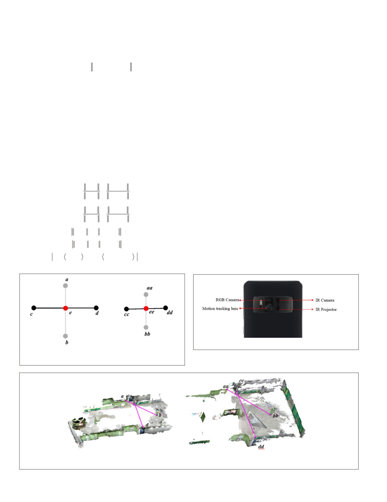
cases (see Figure 3). Letting T = {a, b, c, d} be four coplanar
points selected from a SLAM model, if the four points are not
all collinear, the line ab intersects the line cd at an interme-
diate point e. A corresponding base from a SfM + MVS model
is TT = {aa, bb, cc, dd} with an intermediate point ee. The
invariants and scale constrain the search for reasonable four-
point bases (see Equations 5–9).
r
a e
a b
aa ee
aa bb 1 = -
- ≈ -
- ; (5)
r
c e
c d
cc ee
cc dd 2 = -
- ≈ -
- ; (6)
a b aa bb− − − ≤α ε ; (7)
c d cc dd− − − ≤α ε ; (8)
cos( , ) cos( , ) , ab cd aabb ccdd − ≤ ω (9)
where r1 and r2 are invariant ratios, α is the scale factor, ε,
and ω represent the given thresholds in the distance and
angle measurements, respectively, and áñ is an operator to
calculate the acute angle from crossed lines. Equations 5 and
6 represent the rule that intersection ratios of the diagonals
in an arbitrary planar quadrangle are invariant under affine
transformation (Huttenlocher 1991). Moreover, Equations 7–-9
strengthen geometric constraints for the correspondences in
both the distance and angle measurements. Figure 4 shows
an example of a setup of a four-point set in the SLAM dataset
(left), and one of its corresponding sets in the SfM + MVS data-
set (right).
Experimental Evaluation
Description of the Sensor and the Testing Sites
The performance of the proposed system is evaluated with
two datasets captured from different scenes. We use a Tango
system to capture data (seeFigure 5). Smartphones such as
Tango have built-in RGB and depth sensors, and the maximum
working distance of the depth sensor is about 4 m. In our
cases, the test scenarios are larger than the traditional working
scenes of the RGB-D sensors (that is, indoor applications). The
first dataset was captured along a corridor at a large public
rest area (see Figure 6), and the subsequent test was carried
out in a subway station (see Figure 7). In our experiments, we
captured most of the data in the scenes from along the wall.
Thus, the trajectory of the data collection does not cover the
entire scene, and the middle parts of the scenes are obviously
out of the working range of the depth sensor. Although these
two experiments are specially designed to test and prove
the proposed system, they can also be used to generate an
enhanced 3D model for mapping issues when the trajectories
cannot cover the whole scene or to build a large 3D model for
a more economical approach.
Figure 3. Illustration of the structure of the corresponding
four-point set.
Figure 4. Selection of the four-point sets in the SLAM model (left) and the SfM + MVS model (right).
Figure 5. Hardware scheme of the RGB-D sensor.
636 September 2019 PHOTOGRAMMETRIC ENGINEERING & REMOTE SENSING