terrain coordinates were applied in Equation 8, which is de-
rived from Equation 7 and introduces the
R
B
rotation matrix,
which is a correction to the initial
R
LU
IMU
:
R
g
IMU
(
t
)
–1
*[
r
i
g
–
r
g
LS
(
t
)] =
R
B
R
LU
IMU
r
i
LU
(
t
).
(8)
R
B
is the rotation matrix related to the misalignment cor-
rection in the function of the unknown angles (
d
ω
,
d
φ
,
d
κ
),
given by multiplying
R
Z
(
d
κ
)
R
Y
(
d
φ
)
R
X
(
d
ω
). The elements of
the
R
B
matrix can be estimated by the least-squares method.
The value
r
g
LS
is the laser-unit position in the geodetic refer-
ence system, corresponding to
r
g
GNSS
(
t
) +
R
g
IMU
(
t
)
r
LU
IMU
, and
r
i
LU
(
t
)
is the point position in the laser-unit reference system esti-
mated by
R
ED
LU
(
t
)
ρ
i
(
t
).
Experiments
Data Acquisition
The
UAV
flight was conducted in a test area located inside the
São Paulo State University (UNESP) campus in Presidente
Prudente (22°07
′
S, 51°24
′
W), Brazil. The flight maneuvers
were performed as described under Postprocessing Synchro-
nization to generate the features that enable off-line synchro-
nization.
The flight height was approximately 35 m, with lateral
overlap ranging from 60% to 80% and a flight speed of 4 m/s,
in a north-south direction. In this flight, four flight strips were
collected. Two strips correspond to data acquired during take-
off and landing; the central strips are the interest area to be
mapped. The navigation system was configured with a
GNSS
receiver frequency of 50
Hz
and
IMU
frequency of 125
Hz
. The
UAV
-
LS
system was set up considering an angular aperture of
60° (+30° to −30°) and scan frequency of 25
Hz
, which was
resampled (up-sampled) by linear interpolation to the same
frequency as the
GNSS
receiver. This interpolation was per-
formed to increase the lidar data frequency and to avoid data
losses if
GNSS
observations were downscaled to 25
Hz
. The
original frequencies could also be used in computing correla-
tion, but interpolations would be also necessary.
The raw navigation data were processed using Inertial Ex-
plorer 8.6. The
GNSS
positioning was performed in the relative
mode using a kinematic solution, with
of 8 cm. The platform attitude was obt
accuracy of 0.17° in the heading estim
pitch and roll estimation. The heading standard deviation can
be improved with calibration maneuvers before
UAV
flight.
GCPs
were measured in the test area to estimate the er-
rors affecting the
UAV
-
LS
synchronization and the final point
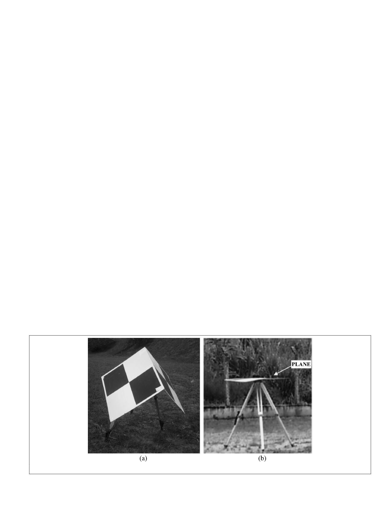
cloud. Different types of
GCP
were used, including two targets
(Figure 3) composed of flat panels. The first target (3D target)
was mounted in pyramidal format, with three flat plates (90 ×
90 cm) painted black and white (Figure 3a), ensuring proper
location in the optical images. The 3D target was designed to
enable accurate estimation of the top of the target on the point
cloud. The second target consisted of a horizontal flat plate
positioned level on a tripod (Figure 3b).
Five
GCPs
were collected with a double-frequency
GNSS
re-
ceiver (Topcon Hiper GGD), and 15
GCPs
were measured using
a tacheometer (Topcon IS robotic total station), which is nec-
essary because
GCPs
around trees and buildings are difficult to
acquire with suitable accuracy with
GNSS
positioning, as it is
influenced by multipath and signal occlusion. Thus, 20
GCPs
were used to perform the point-cloud quality control and fur-
ther corrections. Each
GNSS
control point was tracked during
30 min with an elevation mask of 10° and collection rate of 1
s. The coordinates were calculated with relative positioning
using GrafNet software (NovAtel), achieving an average posi-
tional accuracy of 3 mm. The average positional accuracy of
points measured by tachometry was 5 mm. The distribution
of control points is presented in Figure 4. The points acquired
at building edges are represent in white, and the 3D and plane
targets used for planimetric control are shown in black. The
GCPs
on the ground that were used for altimetric control are
illustrated in gray.
ALS Data Processing and Performance Assessment
Many sources of errors, including both systematic and
random errors, can affect the absolute accuracy of a tridi-
mensional point cloud obtained with the
ALS
system. These
errors can be considered interconnected due to the complex
interrelationships of the
ALS
structure (Shan and Toth 2018).
Therefore, the effects of these errors on the measurements are
difficult to quantify separately. For instance, data synchroni-
zation and
ALS
calibration procedures are indispensable for
generating a suitable
ALS
point cloud, minimizing the main
source of errors that affect the final product. In this regard,
omparative analyses focusing on syn-
cy with correlation,
LSM
refinement, and
the correction of the boresight angles. The
first assessment evaluated the proposed method considering
Figure 3. Targets for quality control: (a) pyramidal and (b) plane on the tripod.
PHOTOGRAMMETRIC ENGINEERING & REMOTE SENSING
October 2019
757


