were obtained; the average, standard deviation, and
RMSE
of
these 13 discrepancies were calculated to estimate the point-
cloud altimetric accuracy.
Point-Cloud Planimetric Quality Control
Planimetric quality control was performed by comparing
the planimetric coordinates of each
GCP
with an interpolated
point obtained from the laser point cloud. This process was
performed using two approaches: point coordinates computed
by line intersections for points collected at building edges
(three
GCPs
) and centroid calculation for geometric targets
such as the 3D and flat-plane targets (four
GCPs
).
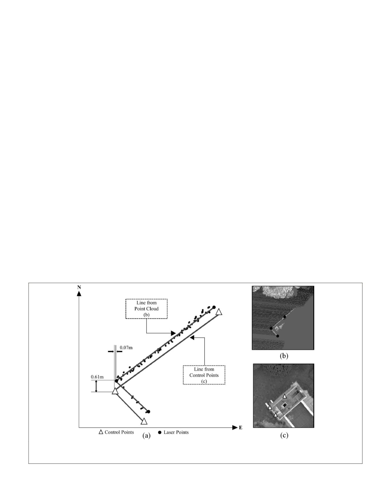
In the first approach, CloudCompare software was used to
select features of interest (building and roof corners) in the
laser point cloud. The point cloud was cropped and exported
to .dxf format. First, horizontal profiles of the points extracted
from the point cloud were created in computer-aided design
software (Figure 5). Since building corners were not well de-
fined in the point cloud, they were determined from straight-
line intersections based on a set of points from the laser point
cloud reaching the building (Figure 5b). Therefore, the coor-
dinates of the building corners in the laser point cloud were
obtained by straight-line intersections. The discrepancies
between building corners measured in the point cloud and
measured directly (from control points; Figure 5c) were com-
puted for planimetric error assessment. These processes will
be automated in future research, with plane fitting followed
by plane intersections. Figure 5a depicts this procedure, in
which the white points represent the control points directly
measured on the building corner and facades with a tacheom-
eter, and the black points show the points extracted from a
horizontal profile of the point cloud.
In the second approach, centroids were calculated using
all points in the laser point cloud belonging to the 2D flat
target (18 points), the 3D target (23 points), and the natural
features—for instance, the light pole (40 points) and the con-
crete pillar (eight points). The points from these targets were
cropped with CloudCompare software and converted to .shp
(shape) format. A convex polygon was fitted for each target,
enabling centroid estimation using
QGIS
(Quantum
GIS
) free
software. The centroids computed were compared with the
GCP
measured in the center of the targets.
Results and Discussion
Postprocessing Synchronization Results: The Estimation of
Clock Differences and LSM Refinement
The clock differences between lidar and
GNSS
measurements
were estimated by cross-correlation function, considering the
lidar data vector as a reference and the vector of
GNSS
data as
the search space. The signal at the beginning of the flight tra-
jectory was compared considering a reference vector contain-
ing 1969 normalized height values, which describes the lidar
signal, and a search vector with 3752 values. The maximum
correlation coefficient obtained between the reference and
search vector was 0.999, resulting in a clock difference of 476
847.812 seconds. At the end of the flight trajectory, a refer-
ence and search vector with 990 and 2608 normalized height
values, respectively, were used, resulting in a maximum
correlation coefficient of 0.9995 and a clock difference of
476 847.77367 seconds. The average value obtained from the
clock differences calculated for takeoff and landing instants
was 476 847.79298 seconds. This difference represents the
raw clock discrepancies between laser time (internal refer-
ence) and
GPS
time given in
GPS
week time. The
GPS
week time
is defined as the number of seconds since the beginning of the
current week, ranging from 0 at the beginning of the week to
604 800 at the end of the week (Seeber 2003).
Figure 6 depicts the heights and clock values converted
to a common time reference, which was the instant when the
devices were turned on, resulting in a difference of 100.36
seconds. Figure 6a and 6b shows the lidar distances obtained
during takeoff and landing, respectively, while Figure 6c and
6d presents the respective
GNSS
flight heights resulting from
the flight maneuvers performed with the
UAV
-
LS
system at the
beginning and end of the flight trajectory. These results were
obtained considering flight maneuvers performed only above
Figure 5. (a) Example of straight-line intersections using (b) points extracted from a horizontal profile of the point cloud
(black points) and (c) aerial view of the ground control points (white points), using building-corner definition for planimetric
error assessment.
PHOTOGRAMMETRIC ENGINEERING & REMOTE SENSING
October 2019
759


