image:
alt
∈
R
w
×
h
at the same spatial resolution as
dsm
. Their
difference generates a discrepancy map (Figure 1c). A base-
line approach is proposed relying on the statistics of pixel
values computed using the
S
functions (Figure 5).
ν
height
(
M
) =
S
(
dsm
–
alt
)
(5)
Equation 5 summarizes how building height-based features
are computed. Different from a root mean square metric (La-
farge and Mallet 2012; Poullis 2013), the histogram captures
the discrepancy distribution, which is particularly helpful in
detecting undersegmentation defects or geometric impreci-
sion. However, as for the previous geometric attributes, the
grid structure of information coming from the model is lost.
Errors cannot be spatialized and linked to a specific facet.
Image-Based Features
We aim to benefit from the high frequencies in Very High Spa-
tial Resolution optical images. Building edges correspond to
sharp discontinuities in images (Ortner
et al.
2007). We verify
this by comparing these edges to local gradients. We start
by projecting building models on the orthorectified image
I
(Figure 6a). For each facet, we isolate an edge
s
(Figure 6b). In
an ideal setting, gradients computed at pixels
g
that inter-
sect
s
need to be almost be collinear with its normal
n
(
s
). In
consequence, applying the same statistics functions
S
, we
compute the distribution of the cosine similarity between the
local gradient and the normal all along that
s
:
D s I S
I g n s
I g
S
g I
g s
,
.
.
( )
∇
( )
( )
∇
( )
∈ ∩ ≠∅
and
(6)
Once the distribution is computed over a segment, it is
stacked over all facet edges to define the distribution over
projected facets. In the case of histograms
S
p
hist
with the same
parameters (and thus the same bins), it is equivalent to sum-
ming out the previous vectors
D
(
s, I
) over edges s from the
projection
q
(
f
) of the facet
f
. In order to take into account the
variability of segment dimensions, this sum is normalized by
segment lengths.
D f I
s D
S
s q f
S
p
p
hist
hist
,
.
( )
∈
( )
∑
The same can be done over all facets of a building
M
(Equation 8). The weights are added in order to take into
account the geometry heterogeneity. The gradient to normal
comparison is similar to the 3D data fitting term formulated
in (Li
et al.
2016). Once again, the model structure is partially
lost when simply summing histograms over all segments.
v
M D M I
q f D f I
S
f F
S
p
p
image
hist
hist
( )
=
(
)
( )
(
)
( )
∈
∑
,
.
,
A
(8)
These image-based attributes are helpful for precision
error detection. As example, facet imprecise borders can be
detected as local gradients direction will be expected to differ
greatly from the inaccurate edge. It can also be detrimental in
under-segmentation detection as colors can change consid-
erably from one facet or one building to another inducing a
gradient orthogonal to edge normals.
Classification Process
Two sources of flexibility are taken into account. First, the
parametric nature of the taxonomy leads to a varying set
of label. Second, the classifier should be able to handle the
ature vector and must adapt to different
d sizes.
We first define two terms used afterwards. In a multiclass
classification problem, each instance has only one label that
takes only one value amongst multiple ones (two in the case
Figure 5. Histogram height-based features computed from the DSM residuals. (a) DSMs. (b) Height maps extracted from the
3D model. (c) Difference between (a) and (b). (d) The difference is transformed into a vector using a histogram.
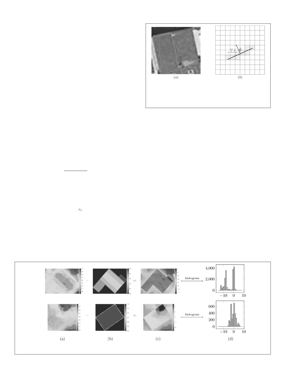
Figure 6. Illustration of how features are derived from
optical images. (a) Model facets (each represented by a
specific color) are projected onto the aerial image. (b) Local
gradients (in purple), on intersecting pixels (in green), are
compared to the edge (in red) normal (in black).
870
December 2019
PHOTOGRAMMETRIC ENGINEERING & REMOTE SENSING


