is depicted in Figure 3.ii.e.2 All these errors stem either
from the modeling approach, or from the poor spatial reso-
lution of the input data (
DSM
or point cloud).
These errors can be related to state-of-the-art labels. For
instance, Missing Node (resp. False Node, Missing Edge,
and False Edge) in Xiong
et al.
(2014) correspond to, or are
included in, the topological atomic errors from the Facet
Errors family:
FUS
(resp.
FOS
,
FIT
, and
FIT
). The difference is
that we distinguish flaws that can affect superstructure facets
(
LoD
-3) from the ones that impair building facets (
LoD
-2).
The taxonomy developed by Michelin
et al.
(2013), on the
other hand, is closer to ours. In fact, while footprint errors is
reshuffled into Building Errors as
BIB
(erroneous outline and
imprecise footprint) and
BIT
(missing inner court) , intrinsic
reconstruction errors (over-segmentation, under segmentation,
inexact roof, and Z translation) can be readapted into both
family errors. Finally, vegetation occlusion and nonexisting
are gathered into the unqualifiable label at finesse level 0.
Boudet
et al.
(2006), however, studied the acceptability of a
model in a whole. Their taxonomy cannot directly fit with our
labels. The acceptability dimension can be incorporated into
our framework by attributing a confidence score to each error:
for example, a prediction probability.
Feature Baseline
In order to detect such specific labels while guaranteeing a cer-
tain flexibility towards reference data, multiple modalities are
necessary. The structure of the 3D model can be directly used
to extract geometrical features. Dense depth information can be
added, through for instance a
DSM
, so as to help detecting geo-
metric defects that can be hardly discriminated otherwise (as in
Figure 3.ii.e), in particular for the outer part of buildings.
VHR
optical images bring additional information (high frequencies
and texture) that is particularly suited for inner defect detec-
tion. Since there is no comparable work that studies the previ-
ously defined errors, we propose a baseline for each modality.
Attributes are kept simple so as to be used in most situations
relying on generally available data. We avoid computing and
comparing 3D lines (Michelin
et al.
2013), correlation scores
(Boudet
et al.
2006) or any Structure-from-Motion based metric
(Kowdle
et al.
2011). In addition of being very costly, these
features are methodologically redundant
techniques: they are vulnerable to the sa
ly, evaluation metrics used in the 3D buil
literature (e.g.,
RMSE
) are too weak for such a complex task.
Geometric Features
The model facet set is denoted by F.
"
(
f,g
)
∈
F
×
F
f
~
g
correspond
to facets
f
and
g
being adjacent: i.e., they share a common
edge. As the roof topology graph in (Verma
et al.
2006), the
input building model
M
can be seen as a facet (dual) graph:
M
=
(
F, E
=
({{
f,g
}
⊂
F:f
~
g
}))
(1)
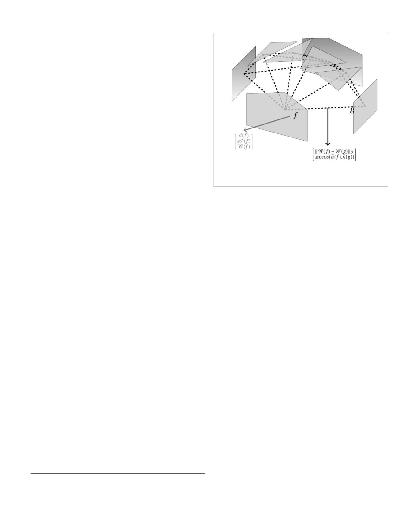
The dual graph is illustrated in Figure 4. For each
facet
f
∈
F
, we compute its degree (i.e., number of vertices;
d
(
f
) =
|{
v
:
v
is a vertex of
f
}|, its area
A
(
f
) and its circumfer-
ence
C
(
f
). For each graph edge
e
= {
f,g
}
∈
E
, we look for the dis-
tance between facet centroids
G
(
f
) –
G
(
g
) and the angle formed
by their normals arccos (
n
(
f
).
n
(
g
)). Statistical characteristics
are then computed over building model facets using specific
functions
S
, like a histogram:
S
=
S
p
hist
:
l
histogram(
l,p
)
(2)
2. There is a problem of slope. The model corresponds to a flat
roof whereas in reality the slope is ca. 25°. The error could only be
shown if we provided the height residual. However, for the sake
of homogeneity, we only provided orthoimages as background. It
motivates also the need for a height-based modality.
with
p
standing for histogram parameters. A simpler option
could be:
S
=
S
synth
:
l
[max(
l
) min(
l
)
l
–
median(
l
)
σ
(
l
)]
(3)
where
l
–
(resp.
σ
(
l
))
represents the mean (resp
.
the standard
deviation) over a tuple.
These features are designed for general topological errors.
For instance, over-segmentation may result in small facet
areas and small angles between their normals. Conversely, an
undersegmented facet would have a large area. Later on, the
importance of these features will be discussed in details based
on experimental results.
Each building
M
can consequently be characterized by a
geometric feature vector that accounts for its geometric char-
acteristics:
v
M
S d f
S f
S f
f F
f F
f F
geometric
( )
=
( )
(
)
( )
(
)
( )
(
)
∈
∈
∈
A
C
( )
−
( )
(
)
( ) ( )
(
)
( )
(
)
{ }
∈
S f
g
S
n f n g f
f g E
f
G G
,
,
.
arccos
g E
{ }
∈
(4)
Additionally, to individual facet statistics, regularity is
taken into account by looking into adjacent graph nodes as in
(Zhou and Neumann 2012). Such features express a limited
part of structural information. Taking this type of information
into account would implicate graph comparisons which are
not genuinely simple tasks to achieve. Since our objective is
to build a baseline, this approach has not yet been considered.
Height-Based Features
For this modality, raw depth information is provided by a
DSM
as a 2D height grid:
dsm
∈
R
w
×
h
3
. It must have been produced
around the same time of the 3D reconstruction so as to avoid
temporal discrepancies. It is compared to the model height
(Brédif
et al.
2007; Zebedin
et al.
2008). The latter is inferred
from its facets plane equations. It is then rasterized into the
Figure 4. Computed geometric attributes represented on the
dual graph, for facets
f
and
g
. The green vector groups the node
(facet) attributes while the blue one shows the edge features.
PHOTOGRAMMETRIC ENGINEERING & REMOTE SENSING
December 2019
869


