of observed features
X
i
(
t
)
∈
R
D
for parcel
i
and for all years
t
= 1, … ,
T
available for training. Likewise, we denote
Y
i
∈
K
T
the ground truth labels for parcel
i
for each observed year
t
= 1, … ,
T
and with
K
the set of all possible labels.
In the section “Temporal Structure”, we present the graphi-
cal model chosen to capture crop rotation. In the section
“Learning”, we explain how the parameters of this model can
be learned from previous
LPIS
editions. In the section “Infer-
ence”, we explain how to use our model to compute predic-
tion of the label of a parcel at a given date.
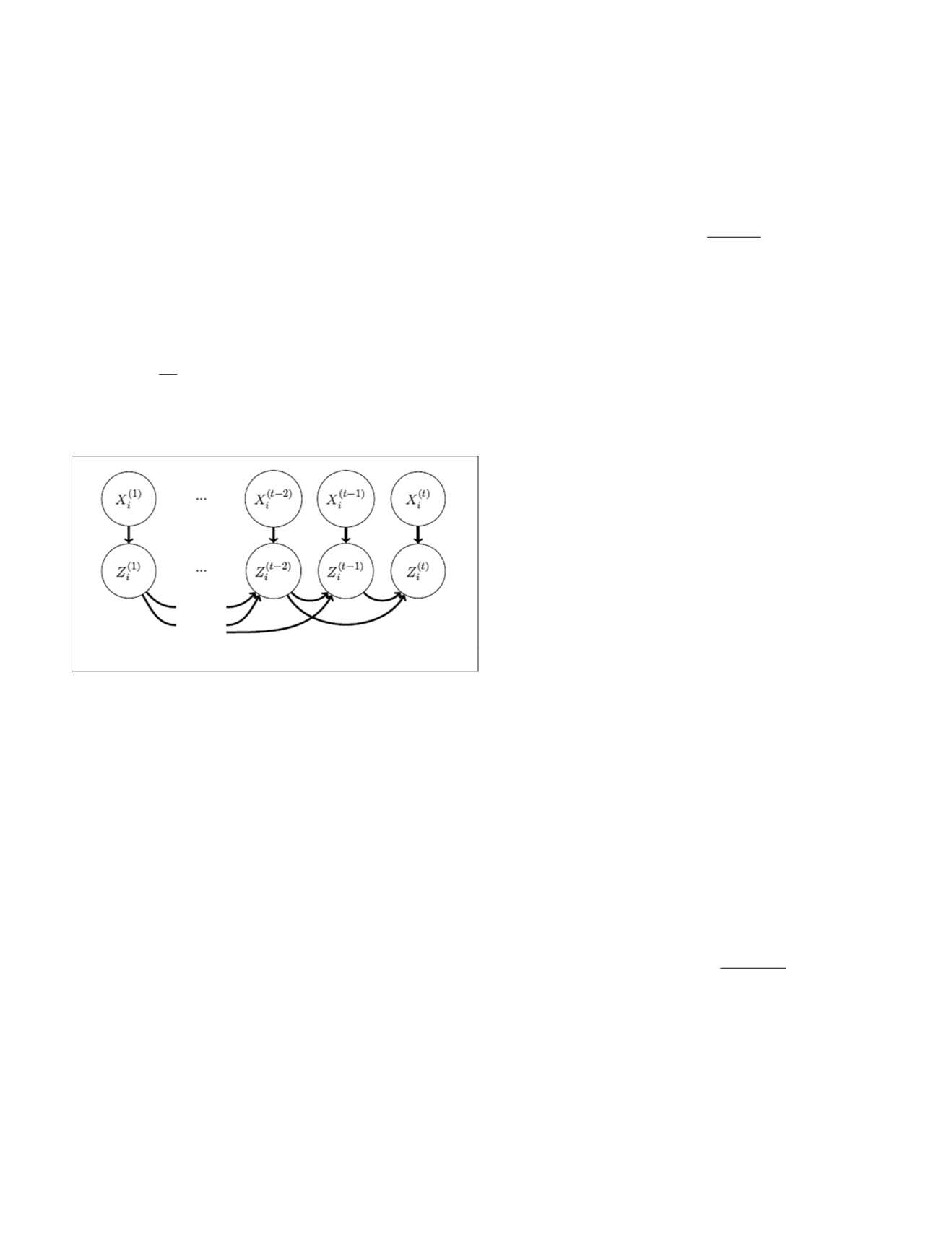
Temporal Structure
The aim of this step is to model the yearly crop rotations in
order to improve crop type prediction. We model this depen-
dency with a linear chain CRF of order
m
, as shown in Figure
8. For a parcel
i
, we model the posterior distribution
P
(
Zi
|
Xi
)
of predicted labels
Z
i
∈
K
T
given the observed features
X
i
as:
P Zi Xi
A
O Z X
I Z
t
T
i
t
i
t m
T
i
t m
( | )
( ,
(
=
+
=
( )
= +
-
(
)
∑
∑
1
1
1
exp
, ,
, ))
…
( )
Z X
i
t
, (1)
where
A
is a normalizing factor,
O
the observation potentials,
and
I
the interaction potentials, described below.
Figure 8. Graph structure of the temporal dependency at order 2.
Observation potential:
The observation potential models
the link between the observed features and the label of each
parcel.
O
(
Z
i
(
t
)
,
X
i
) is taken as the logarithm of
P
RF
(
Z
i
(
t
)
,
X
i
), the
pseudoprobability for parcel
i
at year
t
to be class
Zi
(
t
) given
by the Random Forest classifier, described in the section
“Parcel-Wise Multi-Source Classification”:
O
(
Z
i
(
t
)
,
X
i
) = log
P
RF
(
Z
i
(
t
)
,
X
i
).
(2)
Interaction potential:
This potential models the temporal de-
pendencies between the parcel’s labels at a given year
t
given
the labels at the
m
previous years. We model this potential as
the logarithm of the transition probability
M
(
Zi
(
t – m
), … ,
Z
i
(
t
)
)
from the sequence of
m
previous labels
Z
i
(
t–m
)
, …,
Z
i
(
m
)
, to a la-
bel
Z
i
(
t
)
at the current date (Liu, Song, Townshend
et al.
2008).
For the sake of simplicity, we choose a temporally homoge-
neous parametrization, independent of the observed features,
and shared by all parcels and years:
I
(
Z
i
(
t–m
)
, …,
Z
i
(
t
)
,
X
) = log(
M
(
Z
i
(
t–m
)
, …,
Z
i
(
t
)
))
(3)
with
M
∈
R
K
m+
1
a tensor such that
∑
z
1
, …, z
m–
1
∈
K
m
–1
M
z
1
, …, z
m–
1
, z
m
= 1
for all
z
m
∈
K
, i.e., a stochastic tensor of order
m
. The tensor
M
is referred to as the transition tensor.
Learning
The observation potential is obtained by training the random
forest classifier. A transition tensor
M
ˆ can be learned from
labeled data over past years. Indeed, maximizing the log-like-
lihood in Equation 1 with respect to
z
1
, …,
z
m
∈
K
to
M
yields the following tensor
M
, defined for all
ˆ
, ,
, ,
, ,
M
N
N
z z
z z
z z
m
m
m
1
1
1
1
…
…
…
=
-
(4)
with
N
k
1
, …,
k
m
the number of sequences
k
1
, …,
k
m
observed in
the labeled data for all parcels and all years, and
N
k
1
, …,
k
m
–1
the
number of sequences
k
1
, …,
k
m
–1
observed in the first
T
–1
years, where
T
is the total number of years available for train-
ing. Excluding the last year is necessary to ensure that
M
ˆ is
indeed a stochastic tensor.
To account for the large size of this matrix (|
K
|
m
+1
), and to
prevent numeric issues, we perform a Laplacian smoothing
with
α
= 1 as described in Manning, Raghavan, and Schütze
(2008, chapter 11.3.2)).
Inference
The aim of this step is to predict the label
Z
i
(
t
)
of a given
parcel at year
t
from the observation of the current year,
and knowing its labeling in the
m
previous years. Once the
random forest yielding the observation potential is trained on
all available data, and the transition tensor
M
ˆ estimated, the
prediction is given by:
P Z k Z
X P Z X M Z
i
t
i
t m t
i
RF i
t
i
i
t m
, )
,
,
, ,
(
|
( )
- … -
(
)
( )
-
(
)
=
∝
(
)
×
1
…
-
( )
,
)
Z
i
t
1
(5)
and normalizing the results over
k
∈
K
to obtain a probability.
Experimental Setup
The random forest classifier is composed of 100 decision
trees. The meta-parameters of the forest, such as the maxi-
mum number of attributes considered at each node, are cho-
sen by
k
-fold cross-validation with
k
= 4.
For the temporal structure, spatiotemporal homogeneity
hypothesis allows us to estimate the transition tensor
M
ˆ . For
each study site, we use the geometrically stable parcel blocks
over a period of five years (2010–2014). To decrease the
number of parameters, only first order transitions were used
(transition from one year to the next).
The data is randomly split equally into two distinct train-
ing and testing sets. The model is trained and validated on the
training set while the quality of the model is estimated on the
testing set. The
OA
is used to assess the general performance
of the model. The F-score combines user accuracy (UA, or
precision) and producer accuracy (
PA
, or recall) and allows
estimating the per-class quality. The F-score for a class
C
is
defined as follows:
F-score
C
UA PA
UA PA
c
c
c
c
( )
=
+
2*
*
(6)
To sum up this information, the F-scores are averaged,
with and without weighting by each class cardinality. The
weighted F-scores reduce biases due to imbalanced data. The
results are averaged over 10 runs.
Results
The results are presented on two distinct agricultural sites
(
≥
1250 km
2
), showing different crop types with highly
PHOTOGRAMMETRIC ENGINEERING & REMOTE SENSING
July 2020
435


