and Tucker, 2005), and has been termed the “greening” of the
Sahel. Heumann
et al
. (2007) used amplitudes generated from
a seasonal
NDVI
time series to examine phenological changes
in the Sahel and Soudan regions in comparison to the season-
ally integrated
NDVI
described above. They found that in the
Sahel, increased in seasonally integrated
NDVI
were indeed
associated with increases in the amplitude of the season
NDVI
time-series. Interestingly, in the Soudan, increases in season-
ally integrated
NDVI
were not associated with increases in
NDVI
amplitude, rather with the length of the growing season
.
The statistical analysis of temporal trends requires repeated
testing of remote sensing data against time, resulting in the mul-
tiple comparison problem. In a small review of papers examin-
ing the analysis of the temporal trends of
NDVI
or
EVI
data
1
, it
was found that 28 of 32 of papers reported p-values, while only
one of these accounted for the multiple comparison problem.
Data
A time-series of the
NDVI
for the study area from the Global
Inventory Modeling and Mapping Studies dataset was used
(Tucker
et al
., 2005). This dataset has a spatial resolution of
8 km and a temporal resolution of ten days. The software
TIMESAT was used to generate smooth time-series of the
NDVI
data using Savizky-Golay filtering and to extract growing
season parameters such as the amplitude of the annual growing
season
NDVI
(Jönsson and Eklundh, 2002; Jönsson and Eklundh,
2004). The software was parameterized for eight different zones
based on the
NDVI
time-series of each zones (see Heumann
et
al
., 2007 for more details). Zones that did not exhibit strongly
seasonality (e.g., desert and humid tropical rainforest) were ex-
cluded from analysis. A total of 105,090 pixels were analyzed.
Statistical Analysis
Ordinary least squares regression was used to fit a linear trend
to the inter-annual
NDVI
amplitude for each pixel. Typically,
each trend would be tested for significance individually
(p <0.05). However, since each pixel can be considered a
repeated test of
NDVI
amplitude versus time, the chance of a
false positive result increases with the number of trends. In
this case, the number of tests is very large (i.e., 105,090) and
by chance alone, one would expect at least 5,254 (105,090 *
0.05) “significant” trends to be detected falsely, representing
over 336,288 sq. km. Two methods were used to adjust for the
large number of multiple comparisons: the Bonferroni Correc-
tion and
FDR
, with adjusted p-values, were also computed.
Results and Discussion
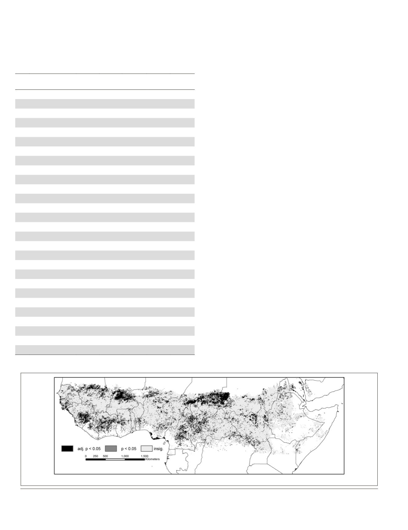
Figure 1 maps the locations of significant linear trends in the
seasonal
NDVI
amplitude using a p-value <0.05 (light blue),
and adjusted p-value <0.05 (dark blue). The results without
correcting for the multiple comparison problem found that
1. From ISI Web of Science using following search terms: - (Remote Sensing AND (AVHRR OR MODIS) AND (NDVI OR EVI) AND trend* NOT classif*)
Figure 1. Significant trends from 1982 to 2005 in the seasonal NDVI amplitude for the Sahelian and Sudano regions of Africa.
T
able
1. L
ist
of
C
orrelation
R
esults
between
I
mage
T
exture
and
G
round
-
based
LAI, S
orted
by
p
-
value
; W
hile
T
hree
M
odels
are
S
ignificant
U
sing
an
U
nadjusted
p
-
value
<0.05 (U
nderlined
)
and
O
ne
M
odel with
an
U
nadjusted
p
-
value
of
<0.01 (
bold
), N
one
of
the
R
esults
are
S
ignificant
after
C
omput
-
ing
the
B
onferroni
C
orrection
(
p
-
value
< 0.0018)
or
F
alse
D
iscovery
R
ate
(
q
-
value
and
A
djusted
p
-
value
S
hown
).
rank
metric
lag
(pixels)
r
p-value
FDR
q-value
FDR adj.
p-value
1
Correlation
7 0.7041 0.0049 0.0018 0.0890
2 Dissimilarity
7 -0.6447 0.0128 0.0036 0.1153
3
Mean
7 -0.5963 0.0244 0.0054 0.1465
4
Mean
3 -0.4928 0.0734 0.0071 0.3301
5
Mean
5 -0.4664 0.0927 0.0089 0.3337
6
Mean
1 -0.4378 0.1174 0.0107 0.3522
7
Correlation
3 -0.4180 0.1369 0.0125 0.3520
8
St. Dev.
1 -0.3938 0.1635 0.0143 0.3679
9 Dissimilarity
5 -0.3916 0.1661 0.0161 0.3322
10
St. Dev.
5 -0.3564 0.2110 0.0179 0.3797
11
St. Dev.
3 -0.3542 0.2140 0.0196 0.3502
12 Inverse Differnce 7 0.3454 0.2264 0.0214 0.3396
13 Dissimilarity
3 -0.3410 0.2328 0.0232 0.3223
14
St. Dev.
7 -0.3322 0.2458 0.0250 0.3161
15
Contrast
1 0.2970 0.3024 0.0268 0.3629
16 Inverse Differnce 3 -0.2311 0.4475 0.0286 0.5034
17 Correlation
5 0.2178 0.4544 0.0304 0.4811
18 Dissimilarity
1 -0.2024 0.4877 0.0321 0.4877
19 Inverse Differnce 5 0.2667 0.4933 0.0339 0.4674
20 Homogeneity
3 0.1914 0.5121 0.0357 0.4609
21
Contrast
5 0.1716 0.5574 0.0375 0.4778
22
Contrast
7 -0.1122 0.7025 0.0393 0.5748
23 Homogeneity
5 -0.1100 0.7081 0.0411 0.5542
24 Correlation
1 0.0792 0.7878 0.0429 0.5909
25 Homogeneity
1 0.0748 0.7994 0.0446 0.5755
26 Homogeneity
7 0.0660 0.8226 0.0464 0.5695
27 Inverse Differnce 1 -0.0616 0.8343 0.0482 0.5562
28
Contrast
3 0.0462 0.8754 0.0500 0.5627
924
December 2015
PHOTOGRAMMETRIC ENGINEERING & REMOTE SENSING


