A
ξ
+
B
(
y + e
) =
d, e
~ (0,
∑
=
σ
2
0
P
–1
)
(7)
where
y
,
e
,
d
,
ξ
, and
P
denote an observation vector, a residual
vector, a constant vector, unknowns, and a weight matrix, re-
spectively; Rearranging Equation 7 leads to the following form:
A
ξ
+
Be
=
w
,
(8)
where
w
=
d
–
By
is a discrepancy vector. Thus, the unknowns
can be derived by Equation 9, and the
a posteriori
standard
deviation of unit weight can be computed using Equation 10,
in which
r
is the number of degrees of freedom (redundancy).
ξ
= (
A
T
(
BP
–1
B
T
)
–1
A
)
–1
A
T
(
BP
–1
B
T
)
–1
w
(9)
σ
0
= ±
e Pe r
T
/
(10)
During the regression, outliers are detected and removed
by leveraging an iterative re-weighting least-squares technique
approach (e.g., Koch 1999; Rangelova
et al
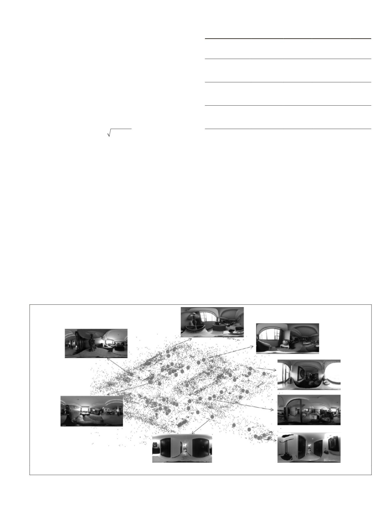
., 2009). Figure
11 depicts a fraction of the 49 indoor images and the recon-
structed results acquired from the proposed method, in which
the small dots and big dots indicate the feature points and the
camera centers.
Table 3 presents the quantitative pose estimation results of
these three methods, in which the posterior standard devia-
tion of unit weight
σ
0
obtained from the least squares adjust-
ment reflects the correctness of the estimation model and
the quality of observations. It can be seen that when solving
49 images (the shortest baselines), each method renders the
most number of feature points and achieves the best accuracy.
As the baselines among the cameras are increased (reducing
the number of images), both performance of each method is
decreased accordingly. Yet, either
PR+SIFT
or the proposed
method outperforms the results of
SURF
in reconstructing
points and camera poses. Also, the proposed rectified spheri-
cal matching seems more robust to long baselines and yields
the best pose estimation result according to the
σ
0
. It shows
possibility in being integrated with the portable panoramic
image mapping system (
PPIMS
) (Tseng
et al
. 2016) to further
improve the accuracy of spherical image pose estimation.
Table 3. Statistic results.
Avg. length
of
baselines
Num. of
images /
Total
Num. of
reconstructed
points
±
σ
0
SURF
(Bay et al., 2006)
0.43 m 47/49
21,459
0.994
1.53 m 17/20
1,903
1.034
2.84 m 10/14
536
1.081
PR+SIFT
(Taira et al., 2015)
0.43 m 49/49
22,174
0.992
1.53 m 20/20
3,688
1.016
2.84 m 13/14
843
1.033
Proposed
method
0.43 m 49/49
23,018
0.992
1.53 m 20/20
3,901
1.009
2.84 m 14/14
869
1.013
Conclusions
This paper contributes a rectified strategy for improving the
matching performance of spherical images. The effectiveness
of this method in yielding stable and well-distributed feature
points regardless of distortion caused by equirectangular pro-
jection has been validated. It can be deemed as a competent
alternative for matching with planar images or establishing
2D-to-3D correspondence with lidar data. In the light of pose
estimation results for a spherical image sequence, the pro-
posed method shows superiority and provides promising re-
sults in dealing with long baseline image pairs. Moreover, the
computational overhead is marginal since it is founded upon
the inherent characteristics of a spherical image and does not
require complex calculations or the generation of additional
rectified images. Thus, it is suitable to be combined with
other recent features such as
SIFT
(Lowe, 2004),
ORB
(Rublee
et
al
., 2011),
CARD
(Ambai and Yoshida, 2011), and BRISK (Leu-
tenegger
et al
., 2011) for further exploitation of imagery.
Currently, the study is coded in Matlab for evaluating
analysis. Promoting the computation efficiency and optimiz-
ing program are always the focuses; however, it is beyond the
scope of this paper.
Figure 11. Reconstructed results and a fraction of images.
PHOTOGRAMMETRIC ENGINEERING & REMOTE SENSING
January 2018
31


