conditions the matching of the grey/black value. Since both
terms are not sufficiently robust for optical flow estimation, a
3
rd
term is introduced that penalizes the total variation of the
optical flow field by a smoothness constraint. Finally, the last
two terms help solve the problem of large displacements by
combining descriptor matching with the variational model
and its coarse-to-fine optimization. The descriptor matching
method is based on densely computed Histogram of Oriented
Gradients (
HOG
). The multiscale approach is performed by
dividing the original problem into a sequence of sub-problems
at different levels of resolution by smoothing the input im-
ages. The levels are defined through a pyramid, where levels
of resolution (k) are down sampled by a factor of 0.95 (kmax-
k), and the kmax is chosen with a discrete derivative filter.
Subsequently, the ultimate goal is to find a function
w(u, v)
that minimizes the energy; it is important to mention that the
minimization is not a trivial task due to the highly nonlinear
model. Brox and Malik (2011) solve this problem by iteratively
updated Euler-Lagrange equations using boundary conditions.
Once the flow field is generated by the optical flow
method, the flow estimation error is estimated for all pairs.
Thereafter, the results are evaluated in a qualitative manner,
where the color-coded flow field is used to show the move-
ment of the glacier. Next, based on Steinbrücker
et al
. (2009),
the consistency of the flow-field for all image pairs is checked
by reconstructing the first image based on the second image
using the estimated motion field
w
according to (Equation 2):
I
r
1
(x) =
I
2
(
x
+
w
(
x
)).
(2)
If the resultant flow is adequate, then the reconstruction
of
I
r
1
has to be nearly identical to
I
1
.
In order to estimate the
error, the absolute difference between the images pairs for the
filtered time-lapse image sequence is estimated by computing
the mean for each pixel.
To obtain the Total Reconstruction Error (
TRE
) of the entire
period, the reconstruction error value per pair (
REp
) is com-
puted for each pixel over the 231 pairs, and then the error
values for two years are estimated by Equation 3. Finally, the
scaling model is applied to convert the values to meters.
TRE
REp
tp
t
axb
n
n
n
=
=
∑
1
231
2*
∆
∆
(3)
where:
axb
is the image size;
REp
n
is the reconstruction error
per pair;
Δ
tp
n
is the time difference between the images in an
image pair; and
Δ
t
is the total time of the study period.
Scaling, Conversion from Image Domain to Object Domain
To obtain the scaled velocity map from the flow field, i.e., to
convert motion in image domain to object space, it is neces-
sary to use a
DEM
to scale the flow parameters at every pixel
of the glacier area.
DEMs
are one of the most common products
in the mapping practice and come in a broad range of spatial
resolutions and accuracy; although their availability greatly
depends on the geographic location.
SRTM
(Shutter Radar Top-
ographic Mission), one of the most popular global
DEMs
, has
coverage in the Viedma glacier area, and, therefore, it was ini-
tially used. Unfortunately the features of the glacier were not
well localized due to the low resolution, 30 m grid, against
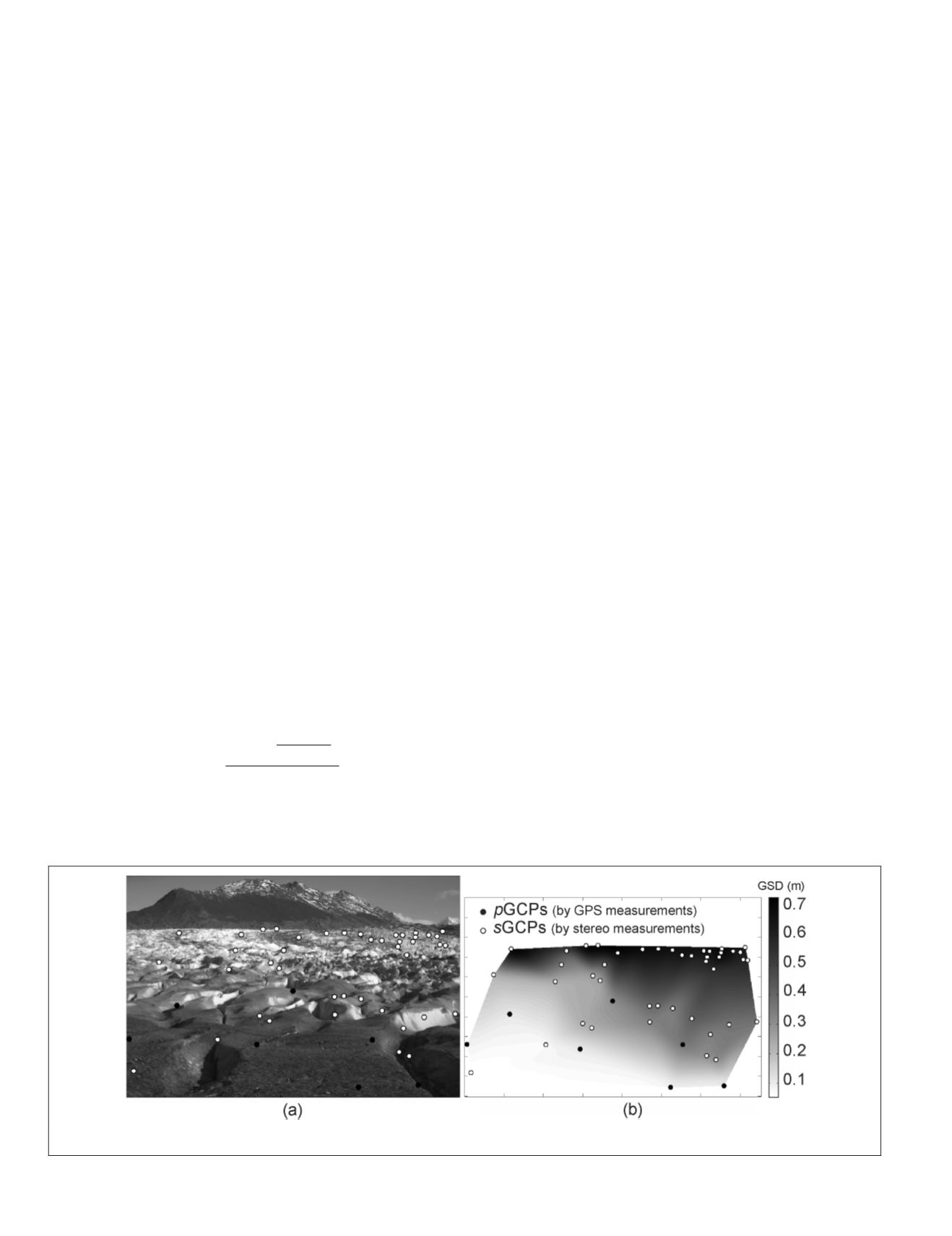
to the about 0.6 m mean Ground Sample Distance (
GSD
) of
the images. Consequently, a sparse
DEM
based on the 50
GCPs
(
p
GCPs
and
s
GCPs
) was generated to convert the optical flow
results in to physical values. In the first step, knowing the
ranges between the C1 and each
GCP
, the
GSD
values for those
GCPs
are estimated. Next, using the
GCPs
an image resampling
is performed by a triangulation method, which is an attrac-
tive interpolator because it can be adapted to various terrain
structures, such as ridge-lines and streams, using a minimal
number of data points (McCullagh, 1988). This method gener-
ates many flat triangles, and is an exact interpolator (Yilmaz,
2007), and thus was chosen because the glacier area is located
in a
zone with relevant topographical details. The spatial
resolution was calculated for the entire glacier area, and the
GSD
ranges value from 0.1 m to 0.7 m, the glacier closest and
farthest extension in the image, respectively. The Root Mean
Square Error (
RMSE
) between the
DEM
and
GCPs
was calculated,
and yielded 0.03 m. Figure 4b shows the distribution of the
GCPs
and resulting
DEM
generated by interpolation.
Results: Motion Detection
On calving glaciers, the velocities can reach a maximum at
the glacier front due to the pulling effect of high calving rates.
These effects are, in particular, amplified when near buoyan-
cy conditions at the front are reached by a glacier calving into
deep waters (Rivera
et al
., 2012a). Very little is known about
the ice flow velocities near the front of Viedma glacier, and
about the ice-lake interactions taking place in this location.
In general, ice flow velocities on a valley glacier cross section
have maximum values at the center of the valley and decrease
down to a minimum at the margins. Along the valley, the ice
velocity magnitude varies longitudinally depending on vari-
ous factors, such as surface slope, mass balance distribution,
and the glacier front conditions.
The velocity field at the lower end of the glacier based on
the scaled
LDOF
results is shown in Figure 5a. The velocity
Figure 4. (a)
GCP
distribution on the glacier surface;
GPS
surveyed, marked by black dots and photogrammetrically derived
ones marked by white dots, and (b)
DEM
created by triangulation method.
38
January 2018
PHOTOGRAMMETRIC ENGINEERING & REMOTE SENSING


