PHOTOGRAMMETRIC ENGINEERING & REMOTE SENSING
March 2018
121
A least squares plane is fit through the neighboring points
using eigenvalue/eigenvector analysis (in a manner similar
to Principal Component Analysis). The equation of the planes
is the same as the component corresponding to the least of
the principal components. The eigenvalue/eigenvector anal-
ysis provides the planar equations as well as the root mean
square error (RMSE) of the plane fit. Single return points in
conjunction with a low threshold for RMSE are used to elim-
inate sample measurements from non-hard surfaces (such
as trees, etc.). The DQM software calculates the offset of the
point (say ´p´) in Swath # 1 to the least squares plane. The
output includes the offset distance, as well as the slope and
aspect of the surface (implied in the planar parameters). It
should be noted that the region that is used to extract planar
features should be “large enough”. It is recommended the ra-
dii of neighborhood be 2-3 times the point spacing. However,
this quantity will be revised in the future as point density of
data increases.
The advantages of using the method of eigenvalues/PCA/
least squares plane fit are fivefold:
a) The RMSE of plane fit provides an indication of the
quality of the control surface. A smaller eigenvalue ratio
indicates high planarity and low curvature. It provides
a quantitative means of measuring control surfaces.
b) Point-to-Plane comparisons are well established as one
of the best methods of registering point cloud.
c) Converting surfaces to intermediate results in (however
small) loss of accuracy.
d) The arc cosine of Z component of eigenvector gives the
slope of terrain
e) The normal vector of the planes are crucial to calculate
the horizontal errors
Vertical, Systematic and Horizontal Errors
The DQM measurements need to be analyzed to extract es-
timates of horizontal and vertical error. To understand the
errors associated with overlapping swaths, the DQM proto-
type software was tested on several data sets with the USGS,
as well as against datasets with known boresight errors. The
output of the prototype software not only records the errors,
but also the x, y and z coordinates of the test locations, eigen-
values and eigenvectors, as well as the least squares plane
parameters.
The analysis mainly consists of three parts
a) The sampled locations are categorized as functions
of slope of terrain: Flat terrain (defined as those with
slopes less than 10 degrees) versus slopes greater than
10 degrees.
b) For estimates of relative vertical error, DQM measure-
ments from flat areas (slope < 10 degrees) are identified:
a. Vertical error measurements are defined as DQM
errors on flat areas
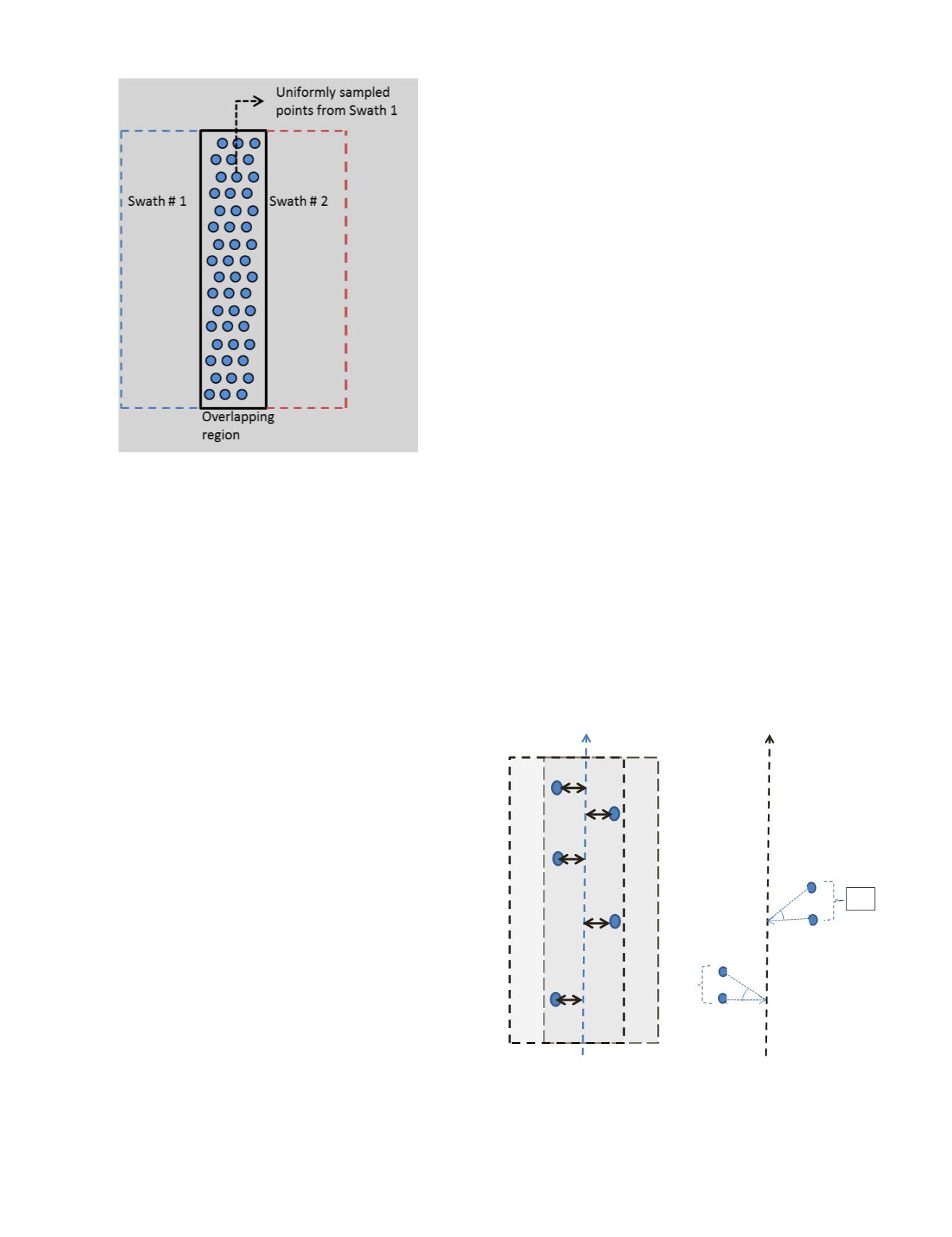
b. For systematic errors, the distance of the above
measured sample check points from center of over-
lap (Dco) are calculated. The center of overlap is
defined as the line along the length of the overlap
region passing through median of sample check
points (Figure 5). The Discrepancy Angle (dSi) (Il-
lustrated in Figure 5) at each sampled location,
defined as the arctangent of DQM error divided by
Dco, is measured
c) The errors along higher slopes are used to determine
the relative horizontal errors in the data as described in
the next section.
Figure 4: Implementation of prototype software for DQM analysis.
Figure 4.pdf 1 2/16/2018 2:51:54 PM
Profile view: Discrepancy Angle s=arc
tangent (dS
i
/D
co
)
ds
i
ds
j
Center of overlap
s
Figure5.pdf 1 2/16/2018 2:52:56PM
Figure: 5 Analysis of DQM errors and center line of overlap.


