126
March 2018
PHOTOGRAMMETRIC ENGINEERING & REMOTE SENSING
This section provides a detailed example of the process of
measuring the vertical, horizontal and systematic accuracy
of two overlapping lidar swaths, without going into the the-
oretical details of performing relative accuracy analysis to
quantify the geometric accuracy of lidar data.
The discrepancies between the overlapping swaths can be
summarized by quantifying three errors between conjugate
features in multiple swaths:
•
Relative vertical errors,
•
Relative horizontal errors and
•
Systematic errors.
The industry uses many ways to measure these errors. Tra-
ditionally, only the relative vertical errors have been quan-
tified, however, there are no standardized processes that
the whole industry uses. Other methods to quantify geomet-
ric accuracy can consist of extracting man-made features
such as planes, lines etc. in one swath and comparing the
conjugate features in other swaths. In case intensity data
are used, the comparisons can also be performed using
2D such as road markings, specially painted targets, etc.
Vertical and Horizontal Error Estimation
To measure and summarize the geometric errors in the data
it is suggested that the following procedure be used.
When multiple swaths are being evaluated at the same time
(as is often the case) the header information in the LAS files
may be used to determine the file pairs that overlap.
For each pair of overlapping swaths, one swath is chosen as
the reference (swath # 1) and the other (swath # 2) is designat-
ed as the search swath. Depending on the user requirements,
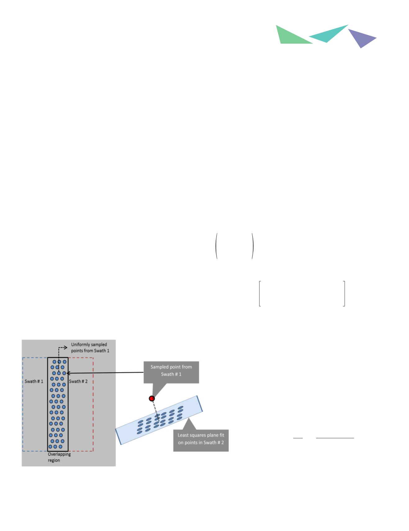
type of area (forested vs. urban/open), 2000points in the over-
lap region of the two swaths are chosen uniformly from swath
# 1. These points must be single return points only. For each
point that has been selected, its neighborhood in swath # 2
is selected. For the point density common in 3DEP, 25 points
can be selected (although this example uses 50 points). Once
the points are selected, a least squares plane is fit through the
points. The distance of this plane from the point swath # 1 is
the measure of discrepancy between two swaths.
The process is explained by means of an example below. As-
suming that we have a point in swath # 1 at the coordinates
(931210.58, 843357.87 and 15.86), Table A.1 lists 50 nearest
neighbors in swath # 2.
T
he first step is to move the origin to the point in swath # 1.
This helps with the precision of the calculations, and allows
us to work with more manageable numbers.
The next step is to generate the covariance matrix of the
neighborhood points. The covariance matrix C is represented
by
σ
2
x
σ
xy
σ
xz
σ
xy
σ
2
x
σ
zy
σ
xz
σ
zy
σ
2
z
where σ
x
, σ
y
, σ
z
are the standard deviations
of x, y and z columns, σ
xy
, σ
xz
, σ
zy
are the three cross correla-
tions respectively. For the points listed in Table A1, the cova-
riance matrix
C
=
4.044 1.006 –1.921
1.006 16.829 –3.087
– 1.921 – 3.087 5.462
.
An eigenvalue, eigenvector analysis of the C matrix provides
the parameters of the least squares fit. In this case, the ei-
genvalues (represented by
λ
1
, λ
2
, λ
3
where
λ
1
> λ
2
> λ
3
) are
respectively (2.48, 9.18 and 25.4).
The eigenvector corresponding to the least eigenvalue of the
covariance matrix represents the plane parameters, and in
this case, the planar parameters are 0.013, -0.026, 0.999, and
-0.054 (represented by Nx, Ny, Nz and D).
The ´D´ value (–0.054) represents the point to plane distance
and is the measure of discrepancy between the swaths at
that location, and is the DQM value at that location. To test
whether this measurement is made on a robust surface, the
eigenvalues can be used to test the planarity of the
location. The ratios:
λ
2
l
1
and
λ
3
l
1
+ l
2
+ l
3
are used
to determine whether the point can be used for fur-
ther analysis. The first ratio has to be greater than
0.8 and the second ratio has to be less than 0.005.
If both the ratio tests are acceptable, the measure-
ment stands.
Figure A.1: Implementation of prototype software for DQM analysis. The plot
on left shows how the overlap regions (single return points only) are sampled
uniformly and the plot on right shows the sampled points from Swath #1 (in
red), its neighbors in Swath #2.
A
ppendix
A: C
alculating
errors
: W
orked
example


