128
March 2018
PHOTOGRAMMETRIC ENGINEERING & REMOTE SENSING
Table A2: A portion (20 measurements) of output file is shown. 10 measurements are from flat regions and 10 are from sloping surfaces.
X
Y
Z
Nx
Ny
Nz
D
Number of
neighbors
280283.61
3363201.64
27.01
0.0338 -0.0249 0.9991
0.2553
1.2774 0.7674 0.0002
16
278544.62
3363296.99
28.44
0.0083 0.0180 0.9998
0.0552
1.2634 0.7100 0.0002
16
275929.96
3363318.85
27.37
0.0168 -0.0034 0.9999
0.1613
1.0022 0.6943 0.0003
14
280581.39
3363373.07
24.28
0.0065 -0.0187 0.9998
-0.0320
0.6607 0.3683 0.0002
18
273856.59
3363385.56
28.66
0.0040 0.0112 0.9999
0.0854
0.7917 0.7423 0.0007
13
279702.17
3363395.30
27.91
-0.0729 0.0333 0.9968
-0.2263
0.7106 0.6454 0.0009
21
274500.56
3363410.55
29.60
-0.0384 0.0157 0.9991
-0.0329
1.0429 0.7272 0.0003
16
273559.31
3363424.17
28.33
0.0370 0.0365 0.9987
0.0652
0.9996 0.5139 0.0012
14
276223.04
3363425.71
30.11
-0.0015 -0.0118 0.9999
-0.0258
0.9276 0.8126 0.0002
18
275747.95
3363450.02
26.44
-0.0405 -0.0450 0.9982
0.1056
0.8210 0.6055 0.0003
16
The rows below have slopes greater than 10 degrees
278928.08
3363230.97
26.86
0.0267 0.2176 0.9757 -0.2744
1.4898 0.7525 0.0002
16
278654.50
3363234.18
28.09
-0.0541 -0.1723 0.9836 0.4879
1.5222 0.7886 0.0002
18
278874.94
3363249.00
24.56
0.0589 0.2005 0.9779 -0.2750
1.4017 0.7269 0.0008
16
278339.98
3363317.26
27.76
0.0730 0.1749 0.9819 -0.1913
1.1565 0.7927 0.0018
16
278572.91
3363325.41
28.15
-0.0710 -0.2039 0.9764 0.4038
1.0060 0.8644 0.0002
16
279167.04
3363349.97
27.74
0.1627 0.1049 0.9811 0.1221
0.8732 0.6538 0.0007
16
278254.99
3363353.27
27.78
0.0718 0.1823 0.9806 -0.1563
0.9359 0.5832 0.0007
14
279152.81
3363380.18
27.60
0.2055 0.0939 0.9741 0.1790
0.9314 0.4998 0.0004
14
278134.66
3363487.79
28.17
0.0766 0.1711 0.9823 -0.3347
0.4553 0.3732 0.0002
22
277950.11
3363503.39
28.53
0.1350 0.1832 0.9738 -0.3548
0.3332 0.2164 0.0002
34
At the end of the process, we have summary estimates (mean,
standard deviation and root mean square error, which is de-
fined as square root of sum of squares of mean and standard
deviation estimates) of error in all the data.
Systematic Error
The systematic errors in the data are quantified by the medi-
an of discrepancy angle. The discrepancy angle is calculated
using the measurements made on flat regions of the overlap-
ping data. A line is fit using the first two columns of Table 2.
In this case, the parameters are: A = – 0.018; B = – 0.999 and
ρ = – 3367777.799. The distances of the points (again first
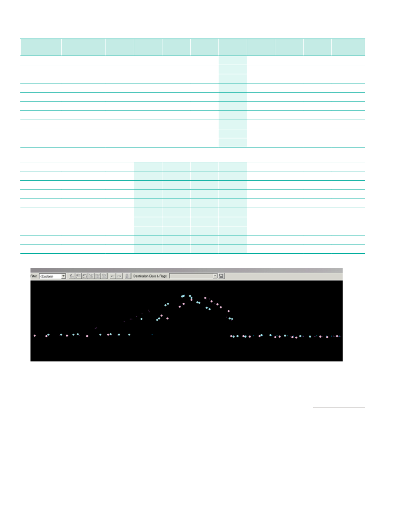
Figure A2: Horizontal Errors in the worked example data set.
two columns of Table A2) from this line are calculated as ρ
D
=
ρ
Distance from Center of Overlap
= |A * X + B * Y – ρ|. The Mean
of discrepancy angle is defined as MDA =
10
∑
i
=1
arctangent
( )
10
Di
ρ
Di
where
Di
are the values in the ´D´ column of Table 2. In this
case, the MDA works out to 0.253 degrees. Nominally, this
value (for a well data set of high geometric quality) is expect-
ed to be close to zero.


