122
March 2018
PHOTOGRAMMETRIC ENGINEERING & REMOTE SENSING
Outliers in the measurements cannot be ruled out. To avoid
these measurements, an outlier removal process using robust
statistics as explained here can be used:
For each category (flat and higher slopes separately), the fol-
lowing quantities can be calculated:
•
DQM
Median
= median(DQM)
z
z
σ
MAD
= Median of |DQM
i
–
DQM
Median
|
•
ZDQM
i
= DQM
i
–
DQM
Median
σ
MAD
•
ZDQM
i
>7, Measurement is an outlier
≤7, Measurement is acceptable
{
Only those points that are deemed acceptable are used for
further analyses. The Median Absolute Deviation method is
only one of many outlier detection methods that can be used.
Any other well defined method would also be acceptable.
Relative Vertical and Systematic Errors
Relative vertical errors can be easily estimated from DQM
measurements made on locations where the slope is less than
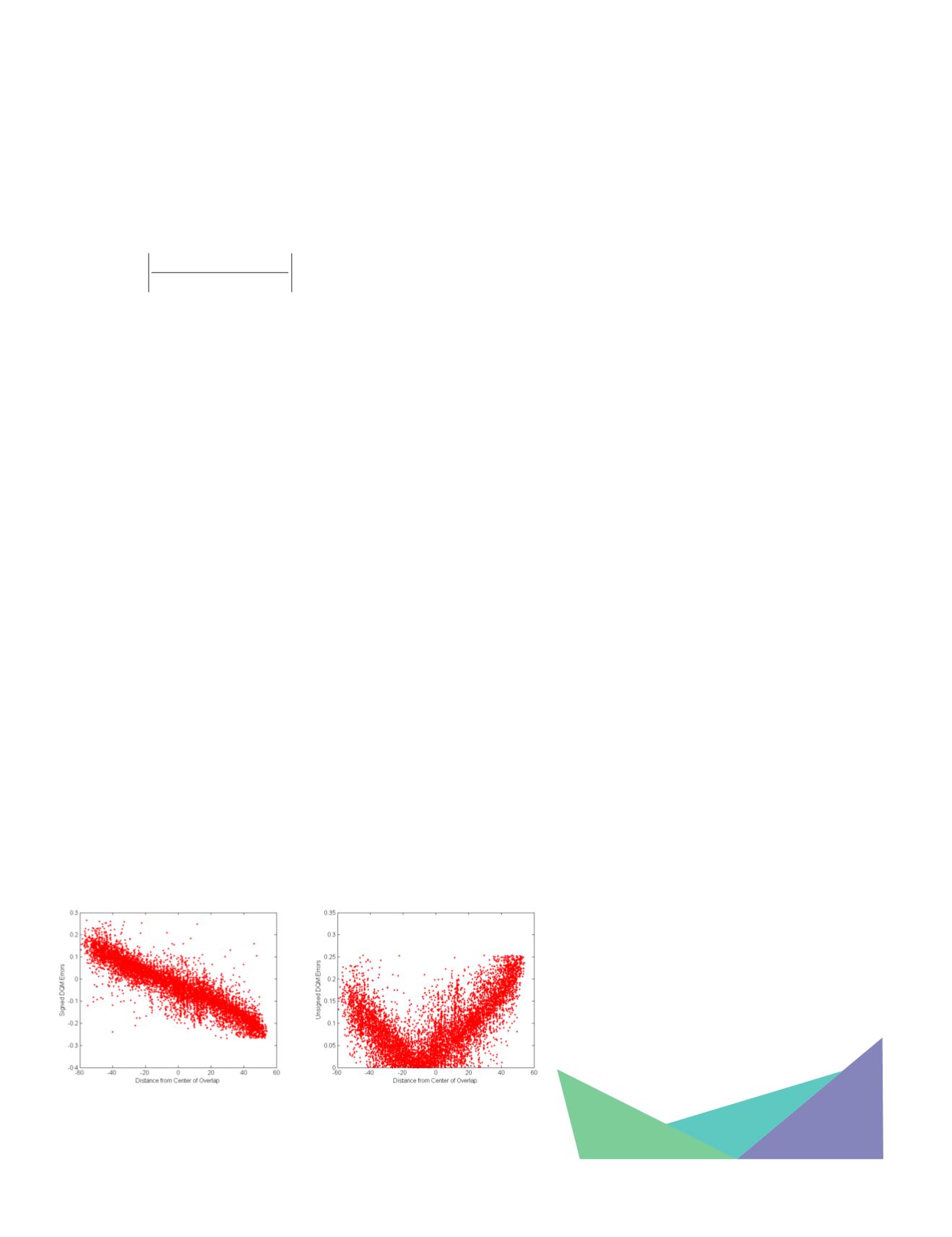
5 degrees (flat locations). Figure 6 shows plot of DQM output
from flat locations as a function of the distance from the cen-
terline of swath overlap.
Positive and Negative Errors:
The analysis of errors based
on point-to-plane DQM can use the sign of the errors. If the
plane (least squares plane) in swath #2 is “above” the point
in swath #1, the error is considered positive, and vice versa.
Figure 6 shows the different methods of representing vertical
errors in a visual manner. Both these methods of representa-
tion of errors can be used to easily identify and interpret the
existence of systematic errors also.
In the presence of substantial systematic errors, relative ver-
tical errors tend to increase as the measurements are made
away from the center of overlap. In particular, errors that
manifest as roll errors (the actual cause of errors may be com-
pletely different) will cause a horizontal and vertical error/
discrepancy in lidar data. Therefore it is possible to observe
these errors in the flat regions (slope less than 10 degrees),
as well as sloping regions. In the flat regions, the magnitude
of vertical bias increases from the center of the overlap. Us-
ing the sign conventions for errors defined previously, these
errors can be modelled as straight line passing through the
center of the overlap (where they are minimal).
In Figure 7, the red dots are measurements taken from flat
regions (defined as those with less than 5 degrees), the green
and the blue dots are taken from regions with greater than
20 degrees slope. The green dots are measurements made on
slopes that face away from the centerline (perpendicular to
flying direction), whereas the blue dots are measurements
taken on slopes that face along (or opposite to) the direction
of flight.
If non-flat regions that slope away from the centerline of
overlap are available for DQM sampling, horizontal errors
can also be observed. It should be noted that the magnitude of
horizontal errors are greater than that of the vertical errors,
for the same error in calibration.
In Figure 7, the first column shows the plot of DQM versus
distance of sample measurements from centerline of overlap.
The consistent and quantifiable slope of the red dots indicates
that Roll errors are present in the data. A regression line is
fitted on the errors as a function of the distance of overlap.
The slope of the regression line defined by the red dots in Fig-
ure 7 is termed Geometric Quality Line (CQL). The slope of
the GQL corresponds theoretically to the mean of all the Dis-
crepancy Angles measured at each DQM sample test point.
In practice, the value is closer to the median of the measured
Discrepancy Angles (perhaps indicating outliers).
Pitch errors cause discrepancy of data in the planimetric co-
ordinates only, and the direction of discrepancy is along the
direction of flight. The discrepancy usually manifests as a
constant shift in features (if the terrain is not very steep).
This requires them to be quantified using measurements
made from non-flat/sloping regions. Figure 7 shows that this
can be achieved (blue dots in the second column indicate pitch
errors) using the DQM measurements. The blue dots indicate
that there is a constant shift along the direction of flight. The
presence of red dots close to the zero error line (and following
a flat distribution) indicates that these errors are not mea-
surable in flat areas. The presence of green dots closer to the
zero line also indicates that pitch errors are not
measurable in slopes that face away from the
flight direction.
The third column in Figure 7 indicates that
when these errors are combined (as is almost
always the case), it is possible to discern their
effects using measurements of DQM on flat and
sloping surfaces.
Figure: 6 Visual representations of systematic errors in the swath data. The plots
show DQM errors isolated from flat regions (slope < 5 degrees). 6(a) plots signed
DQM Errors vs. Distance from the center of Overlap, while 6(b) plots Unsigned DQM
errors vs. Distance from center of overlap.


