where
I
and ˆ
I
are two images to be compared.
α
,
β
,
γ
are
control parameters for adjusting the relative importance and
C
l
(
I
, ˆ
I
),
C
c
(
I
, ˆ
I
),
C
s
(
I
, ˆ
I
) are comparison functions on luminance,
contrast and structure, respectively. Specific introduction of
C
l
(
I
, ˆ
I
),
C
c
(
I
, ˆ
I
),
C
s
(
I
, ˆ
I
) can be found in Wang
et al.
(2019).
The range of
SSIM
is [0:1]. With higher
SSIM
, the recon-
structed images are more similar to the real
HR
images.
Although there is not a specific range of
PSNR
, it follows the
same trend with
SSIM
, which means the higher
PSNR
indicates
better image quality.
For the evaluation of
DSM
quality, two indicators are used
in this paper, namely root-mean-square error (
RMSE
) and mean
relative error (
MRE
). Suppose the reference
DSM
as
D
and the
DSM
from reconstructed images as
C
, so that
D
and
C
are two compo-
nents that need to be compared.
RMSE
and
MRE
for
DSM
quality
assessment can be expressed as Equations 4 and 5, respectively.
RMSE
C D
N
C D
i j
i n j n
ij
ij
,
,
,
,
(
)
=
−
(
)
= =
= =
∑
1
1 1
2
(4)
MRE
C D
N
C D
D
i j
i n j n
ij
ij
ij
,
,
,
,
(
)
=
−
= =
= =
∑
1
1 1
(5)
where
N
stands for the number of a
DSM
matrix’s element, and
(i, j) represents the position at
i
th
row and
j
th
column. To mea-
sure the performance difference of the different
SR
models,
RMSE
and
MRE
between reconstructed
DSMs
and the reference
DSM
are calculated. The lower
RMSE
and
MRE
indicate that the
reconstructed
DSM
is more similar to the reference
DSM
, which
are regarded as a better
DSM
.
Experiments
This section constructs simulated and real data experiments
to verify the feasibility and practicability of the proposed
method for subpixel
DSM
generation. It can be divided into
three subsections, namely experiment details of image
SR
,
simulated experiments, and real data expe
Experiment Details of Image SR
This subsection aims to describe the details of stage I of the
proposed method and compared the results of reconstructed
HR
images.
Training Details
To train these
SR
models, an augmented training dataset was
used. The training dataset contained 291 natural images in
(Schulter
et al.
2015) and 109 very high-resolution aerial
images from the Dataset for Object deTection in Aerial im-
ages (DOTA) dataset (Xia
et al.
2018). The mixed dataset was
randomly split into 1 325 000 standard image patches for
training. Moreover, to ensure the size of the output images un-
changed, symmetric padding was added before each convolu-
tion layer to refine these
CNN
-based
SR
methods. The training
process was implemented on Caffe Library (Wen
et al.
2016).
Image Reconstruction
With the trained models, the
LR
aerospace images were taken
as input to obtain reconstructed
HR
images. Specifically, as
remote sensing images were always in huge size, it was neces-
sary to divide them into patches for practical use. After that,
the reconstructed
HR
images would be merged back according
to their original order. Besides, the image reconstruction pro-
cess was based on MatConvNet (Vedaldi and Lenc 2015).
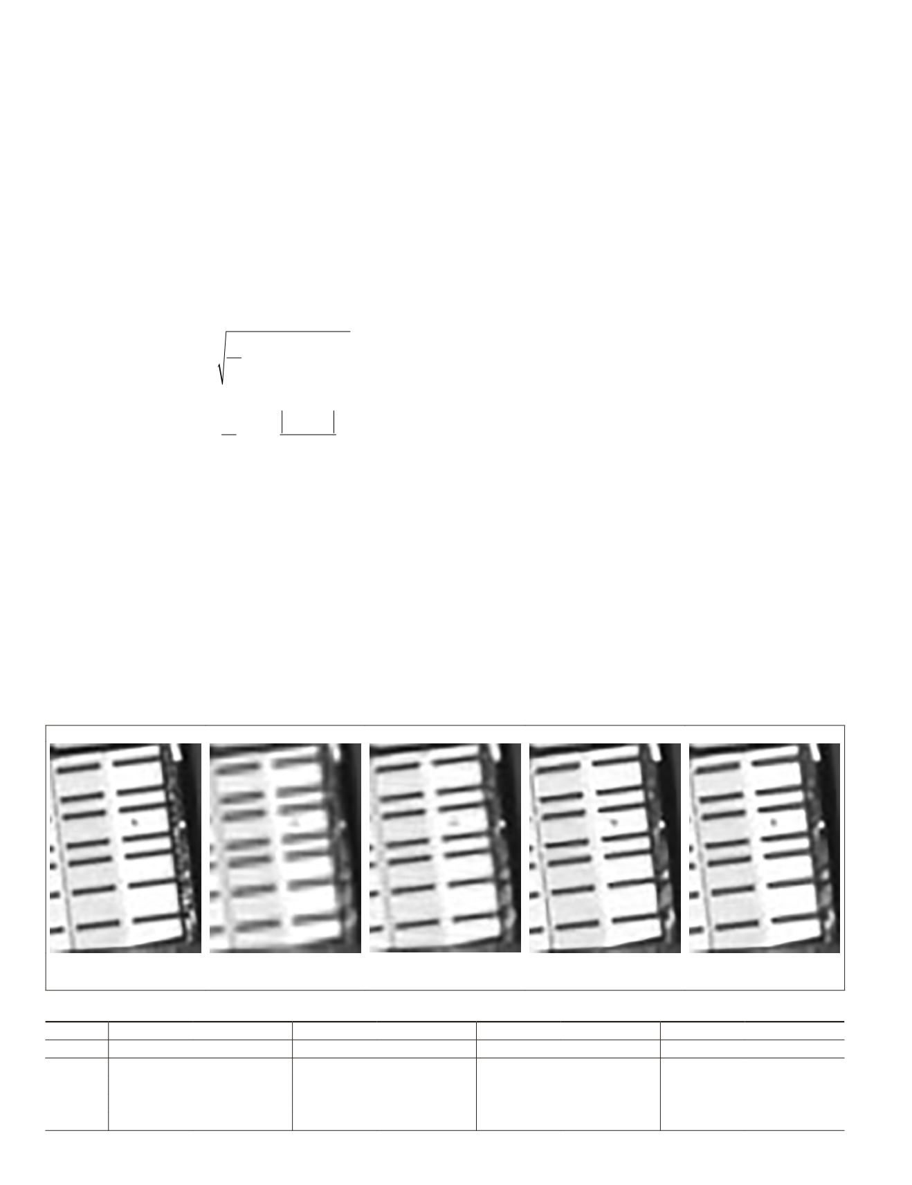
Results Comparison of Super-Resolved Images
To show the texture difference of the reconstructed images, a
building was selected and enlarged to show the visual differ-
ence of the super-resolved images in Figure 3. Besides, several
regions from our tested image dataset were selected to present
the performance difference of these
SR
models, and the quan-
titative
PSNR
and
SSIM
results were shown in Table 1. From
the visual difference of the red ovals in Figure 3, it could be
found that some small objects/texture could be reconstructed
correctly with
VDSR
and
SRMD
, while bicubic and
SRCNN
could
not obtain the same result. And the statistical evaluation fur-
ther showed that
SRMD
outperformed the other methods, while
bicubic performed worst. It was worth noting that the image
texture was of significance in the subsequent image matching
process, so it could be forecasted that with a better
SR
model,
the quality of the corresponding
DSM
would be better.
Ground Truth
Bicubic
SR
SRMD
Figure 3. Visual comparison of the reconstruction results among different SR models (the red ovals: reconstruction results of
a small object on the building roof).
Table 1. Stereo images quality assessment (left/right).
Method
Bicubic
SRCNN
VDSR
SRMD
Regions
PSNR
SSIM
PSNR
SSIM
PSNR
SSIM
PSNR
SSIM
A 29.98/32.28 0.8172/0.8453 32.15/35.21 0.8832/0.9135 33.50/36.99 0.9235/0.9609
34.79/37.66 0.9696/0.9754
B 34.35/34.95 0.7728/0.8679 36.03/37.49 0.7977/0.9246 38.50/37.87 0.9040/0.9617
39.00/38.92 0.9759/0.9699
C 38.75/38.14 0.7405/0.8278 39.73/40.15 0.7382/0.9130 41.42/41.00 0.9146/0.9639
42.40/42.47 0.9772/0.9699
D 40.10/37.09 0.5932/0.8770 40.41/39.20 0.6740/0.9147 43.10/39.80 0.8828/0.9582
44.25/40.05 0.9864/0.9628
768
October 2019
PHOTOGRAMMETRIC ENGINEERING & REMOTE SENSING


