Final Depth Regularization
Given the initial depth, edge cues, and occlusion cues, we
regularize the depth map with an
MRF
. The final depth map is
obtained by minimizing the energy function:
l
l x y l x y
E l x y l x y
l
d
x y
final
smooth
argmin
=
(
)
−
(
)
+
(
) (
)
(
)
′ ′
∑
,
,
, ,
,
,
λ
′ ′
(
)
∈
(
)
∑
x y
x y
,
,
N
, (23)
where
N
(
x,y
) are the neighboring pixels of (
x,y
) and
λ
is a fac-
tor to control the smooth term. The first term in Equation 23
is the data term. The smooth term means the smoothness con-
straint of the adjacent pixels. Similar to in Zhu
et al.
(2017),
the smooth term is defined as
E l x y l x y
l x y l x y
smooth
, ,
,
,
,
(
)
′ ′
(
)
(
)
=
(
)
− ′ ′
(
)
ϖ
(24)
ϖ
σ
=
−
(
)
−
′ ′
(
)
−
(
)
− ′ ′
(
)
exp
Occ
Occ
occ
e
e
x y
x y
I x y I x y
,
,
,
,
2
2
2
2
2
2
2
2
2
σ
σ
e
−
(
)
− ′ ′
(
)
I x y I x y
,
,
, (25)
where
I
e
is the edge map of the center-view image,
I
is the
center-view image,
ϖ
is a weighting function used to pre-
serve sharp occlusion boundaries, and
σ
occ
,
σ
e
, and
σ
are three
weighting factors (set to 1.6, 0.8, and 0.08, respectively, in our
experiments). The minimization is solved using a standard
graph-cut algorithm (Boykov, Veksler, and Zabih 2001).
Experimental Results
In this section, we first show the results of different stages of
our algorithm, then demonstrate the advantages of our algo-
rithm by comparing with different state-of-the-art algorithms.
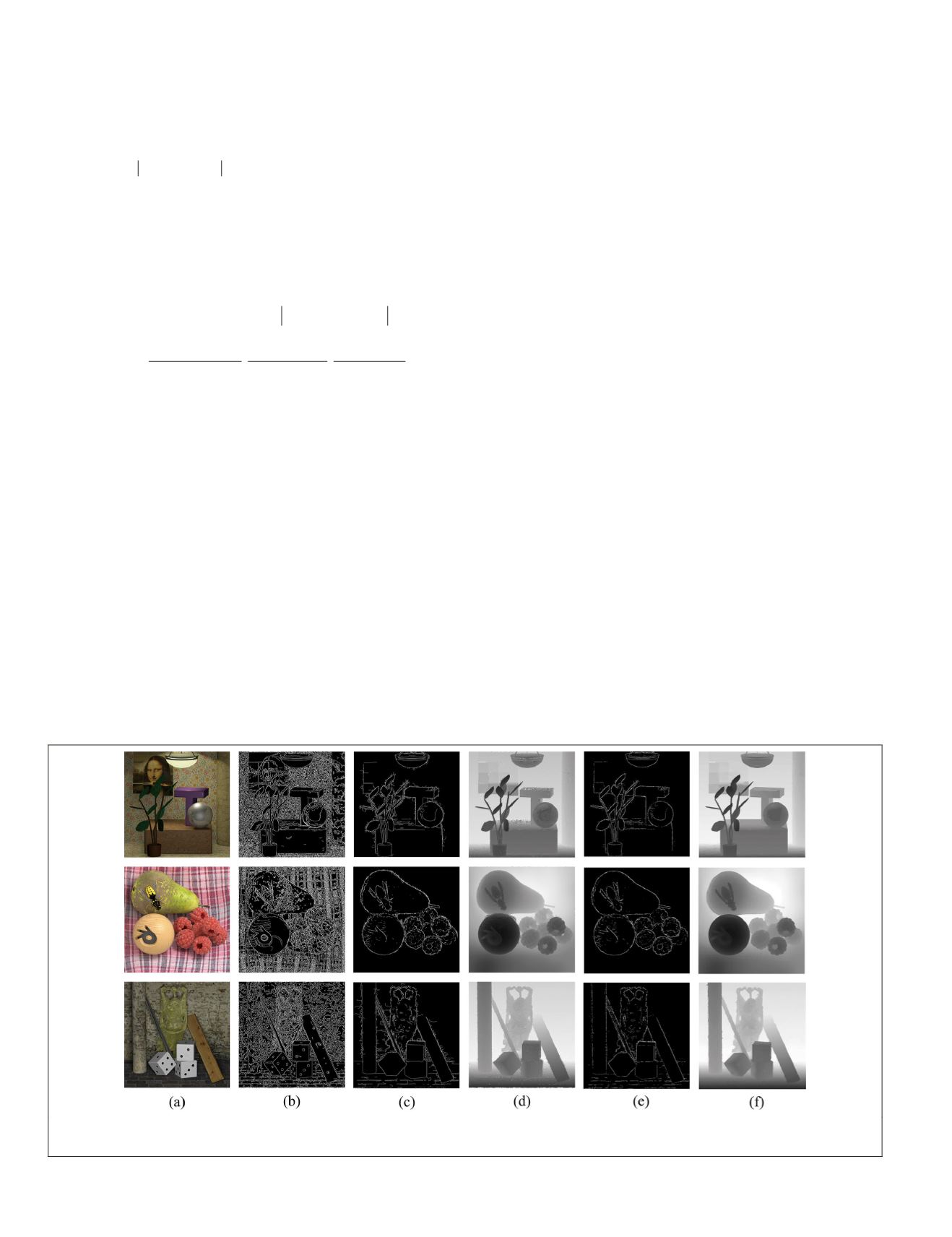
Algorithm Stages
The results of different stages of our algorithm are shown in
Figure 17. First, edge detection is applied on the center-view
image (Figure 17a) to find the initial occluded pixels (Figure
17b). There are many unoccluded pixels in the edge obtained.
We identify the occluded pixels from the edge using the refo-
cusing method (Figure 17c). Then the initial depth is com-
puted (Figure 17d) and the occlusion boundaries are detected
using the method previously explained (Figure 17e). Finally,
given the initial depth and occlusion cues, we regularize the
depth with an
MRF
for a final depth map (Figure 17f).
Comparisons
We compare our results with those of the algorithms by Tao
et al.
(2013), Jeon
et al.
(2015), T.-C. Wang
et al.
(2016), and
Zhu
et al.
(2017) on synthetic data sets created by Wanner
et al.
(2013) and real-scene data sets captured by the Lytro
Illum camera. The results of these algorithms can be obtained
by running their public codes. In addition, we compare our
method with several top-ranked methods from publications
on the 4D Light Field Benchmark (Honauer
et al.
2017),
OBER
-
cross+
ANP
(Schilling
et al.
2018), Epinet-fcn-m (Shin
et al.
2018), and LFattNet (Tsai
et al.
2020) on the training sets in
the 4D Light Field Benchmark.
Synthetic Data-Set Results
The qualitative comparisons of the depth map on the data
sets from Wanner
et al.
(2013) are shown in Figure 18. As we
can see from the figure, the method of Tao
et al.
always gives
oversmooth results in the occlusion boundaries and generates
thicker structures than the ground truth. The method of Jeon
et al.
provides good results for some occlusion boundaries
(the branches in Figure 18a and the close-up of the red box in
Figure 18c) but gives no solution to dealing with occlusion,
due to the lack of an occlusion model. Therefore, some occlu-
sion boundaries are still oversmoothed, such as the close-ups
in Figure 18b and 18d. The method of T.-C. Wang
et al.
can
perform well in single-occluder areas, but it always provides
oversmooth results in multi-occluder areas. The method of
Zhu
et al.
can select more accurate unoccluded views than
the method of T.-C. Wang
et al.
in multi-occluder areas, so it
achieves better results on the depth map; however, it can se-
lect some occluded views in complex-textured regions, which
leads to oversmoothing in the occlusion areas (the branches
in Figure 18a and the close-up of the red box in Figure 18c).
Compared with the state-of-the-art algorithms, our pro-
posed method yields sharper occlusion boundaries in the
depth map. Our method finds more accurate occluded pixels,
illustrated in close-ups of the green box in Figure 18b. The
edge pixels of the black dots on the dice are identified as
Figure 17. The results of our algorithm at different stages on synthetic data sets: (a) Center-view images, (b) edge detection, (c)
occluded pixels, (d) initial depth, (e) occlusion-boundary detection, and (f) final depth.
450
July 2020
PHOTOGRAMMETRIC ENGINEERING & REMOTE SENSING


