Finally, the occluded pixels are identified based on the
discriminant formula
α α δ
1
2
*
*
− >
,
(9)
where
δ
is a threshold value which is set to 5.
Some pixels which are not located in the edge are occlud-
ed in some views of the angular patch, as shown in Figure 10.
In order to identify such occluded pixels, the final occluded
pixels are obtained by dilating the occluded pixels identified.
An example of occluded-pixel identification is shown in
Figure 11. Obviously, using our proposed method removes
a number of unoccluded pixels compared with the methods
of T.-C. Wang
et al.
(2016) and Zhu
et al.
(2017). It can avoid
selection of unoccluded views for unoccluded pixels and thus
ensure the accuracy of depth estimation of the unoccluded
pixels.
Unoccluded-View Selection
Because the photo-consistency assumption only holds for un-
occluded views for occluded pixels, in this section unocclud-
ed views are selected for occluded pixels, which will be used
for depth estimation of occluded pixels in the next section.
For the occluded pixels, the angular patch corresponds to the
spatial patch according to the occluder consistency. There-
fore, the angular patch can be divided into the same regions
as the spatial patch. For some occluded pixels in a complex
scene, spatial patches are divided into multiple regions, and
the corresponding unoccluded views may correspond to a
combination of several regions in the spatial patches. In order
to obtain the optimal unoccluded views, an adaptive unoc-
cluded-view selection method is proposed.
First, the spatial patch of each occluded pixel is divided
into different categories by ty affinity-propagation clustering
(Frey and Dueck 2007), an adaptive clustering algorithm that
does not specify the number of clusters. Instead, the prefer-
ences
p
influence the final number of clusters. Usually a good
choice is to set
p
to the median of all the similarities between
data points. However, in many cases that setting cannot lead
to an optimal clustering solution. According to experimental
experience, we set
p
to two-thirds of the minimum of all the
similarities between data points. The clustering result is gen-
erally two or three categories. If the spatial patch is divided
into two categories, the pixels in one region that share the
same label with the center pixel are labeled as the unoccluded
points; the corresponding views in the angular patch are la-
beled as unoccluded views, as shown in Figure 12. If the spa-
tial patch is divided into three categories, we mark the pixels
sharing the same label with the center pixel as region 1 and
Figure 10. Occlusions around occlusion edges. The left
image is the close-up of the center subaperture image, and
the right images are the angular patches when the red and
blue dots in the close-up image are refocused at the correct
depth. The red dot is located on the occlusion edge of the
center subaperture image, and its corresponding angular
patch is divided into two parts on average. The lower right
part is all from the unoccluded red dot, whereas the upper
left part is occluded by the leaf. The blue dot is located
around the occlusion edge, and some views in the upper
left corner of its angular patch are also occluded.
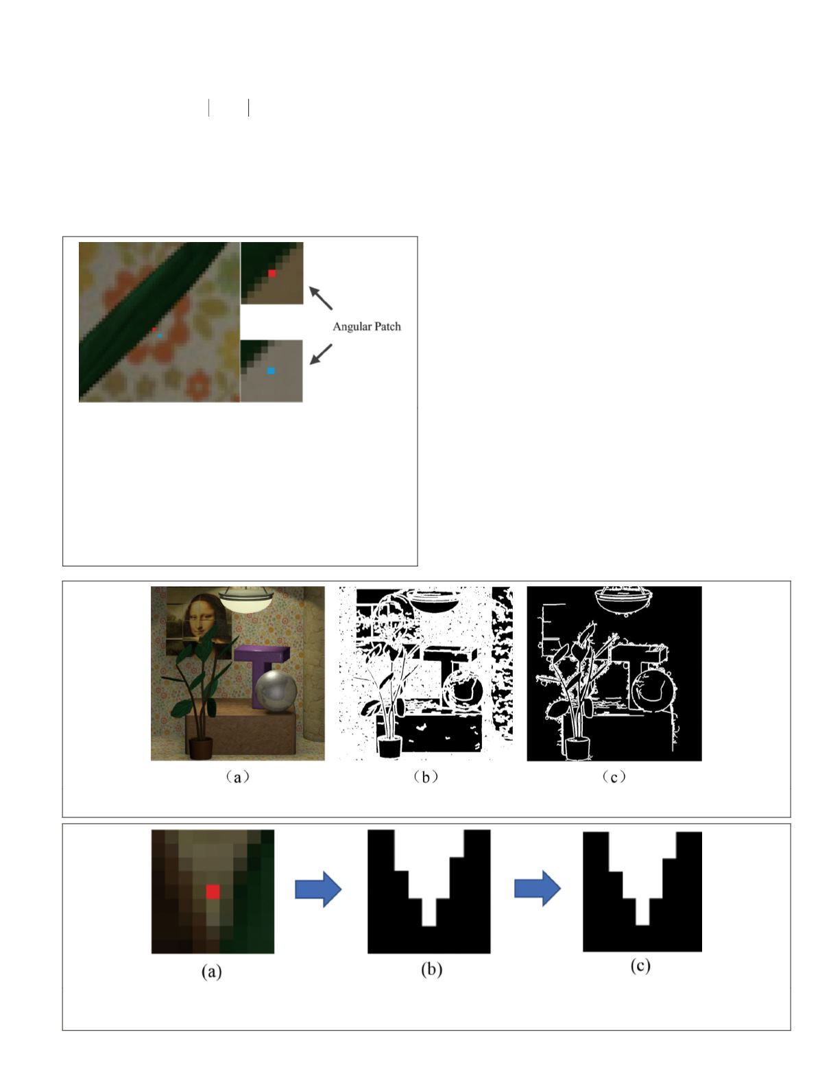
Figure 11. Identification of occluded pixels. (a) The center-view image of the Mona data set (Wanner
et al.
2013). (b) The
occluded pixels identified with the methods of T.-C. Wang
et al.
(2016) and Zhu
et al.
(2017). (c) Our occluded pixels.
Figure 12. Selection of unoccluded views (two categories). (a) The spatial patch of one occluded pixel in the center
subaperture image. (b) Two categories that the spatial patch is divided into. The pixels that share the same label with the
center pixel are shown in white. (c) The angular patch. The corresponding unoccluded views are shown in white.
PHOTOGRAMMETRIC ENGINEERING & REMOTE SENSING
July 2020
447


