method is lower than those from other methods, further verify-
ing the effectiveness of our method. The quantitative compari-
sons of the root-mean-square (
RMS
) errors of the depth maps are
listed in Table 2. As can be seen from the table, our proposed
method is superior to other advanced algorithms in accuracy:
The
RMS
error decreases by about 15% with our proposed
method compared with the best of the four other methods.
Table 2. Root-mean-square error (pixels) of depth maps.
Data Set
Method
Mona Buddha StillLife Horse
Tao
et al.
(2013)
0.189 0.186 0.260 0.202
Jeon
et al.
(2015)
0.087 0.110 0.193 0.155
T.-C. Wang
et al.
(2016)
0.077 0.081 0.171 0.093
Zhu
et al.
(2017)
0.082 0.112 0.113 0.103
Ours
0.063 0.069 0.095 0.065
The qualitative comparisons of the depth map on training
data sets from the 4D Light Field Benchmark are shown in
Figure 20. Our method achieves similar visual results to the
top-ranked methods.
The quantitative comparisons of the depth map are shown
in Table 3. Compared with conventional methods, our method
is superior in terms of mean square error to
OBER
-cross+
ANP
on the Boxes, Cotton, and Dino data sets, but inferior on the
Sideboard data set. Compared with deep-learning methods,
our method outperforms only Epinet-fcn-m on the Boxes data
set, and m underperforms Epinet-fcn-m and LFattNet on the
other data sets. However, both of those methods take about
one week to train the networks on an Nvidia
GTX
1080Ti
graphics processing unit. The average running time of our
algorithm is 1027 s. If you do not have a graphics processing
unit and want to get the disparity map quickly, we think our
approach is a good choice.
Table 3. Mean square error of disparity maps.
Data Set
Method
Boxes
Cotton
Dino Sideboard
OBER
-cross+
ANP
4.750
0.555
0.336
0.941
Epinet-fcn-m 5.967
0.197
0.157
0.798
LFattNet
3.996
0.208
0.093
0.530
Ours
4.474
0.545
0.332
0.972
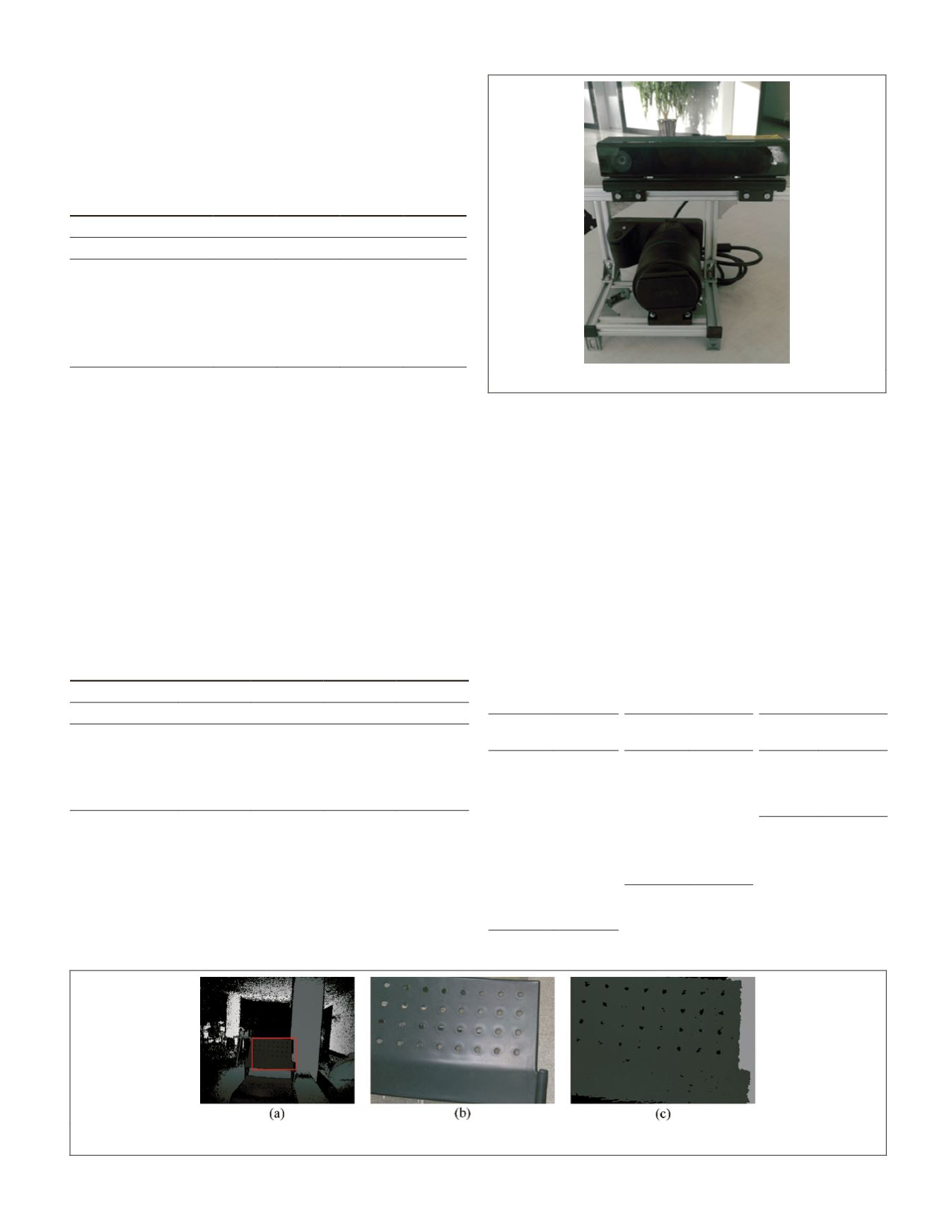
Real-Scene Results
In order to further verify the effectiveness of our proposed
method, experiments were conducted on real-scene images
captured with the Lytro Illum camera. The disparities of the
images range from −1.1 to 1.1. In order to get the ground truth
of the scenes, we fixed an
RGB-D
camera (Kinect 2.0) on the top
of the camera as shown in Figure 21.
First, the Lytro Illum camera was calibrated with check-
erboard patterns using the Camera Calibration Toolbox for
MATLAB
(
)
to get the interior parameters, as shown in Table 4, and sub-
aperture images. Then the infrared camera of the
RGB-D
sensor
was calibrated with checkerboard patterns to get the interior
parameters as shown in Table 5. Finally, stereo calibration
was performed between the center subaperture images and
the infrared camera images by fixing the interior parameters
of the two cameras to obtain the relative pose of the infrared
camera with respect to the Lytro Illum camera, as shown in
Table 6. After the calibration procedure, we registered the
depth maps to the center subaperture image to get the ground
truth of the scenes, as shown in Figure 22.
Table 4. The
interior parameters
of the Lytro Illum
camera.
Table 5. The
interior parameters
of the infrared
camera.
Table 6. External
parameters of the
two cameras.
Parameter Value
Parameter Value
Rotation
Angle (°)
Translation
(mm)
K
1
−13.682
f
x
(pixels) 371.022 0.0165 37.0562
K
2
(mm) 17457.348
f
y
(pixels) 370.187 −0.0057 −135.3635
f
x
(pixels) 18935.380
c
x
(pixels) 254.828 0.0158 −61.0438
f
y
(pixels) 18915.222
c
y
(pixels) 207.339
c
x
(pixels) 3566.461
k
1
0.108
c
y
(pixels) 2720.078
k
2
−0.302
k
1
0.472
k
2
−1.094
Figure 21. The Lytro Illum camera and RGB-D camera.
Figure 22. Obtaining the ground truth. (a) The depth map obtained by the Kinect camera. (b) The center subaperture image.
(c) The ground truth of the center subaperture image.
PHOTOGRAMMETRIC ENGINEERING & REMOTE SENSING
July 2020
453


