the occluded pixels from the edge pixels using a refocusing
method.
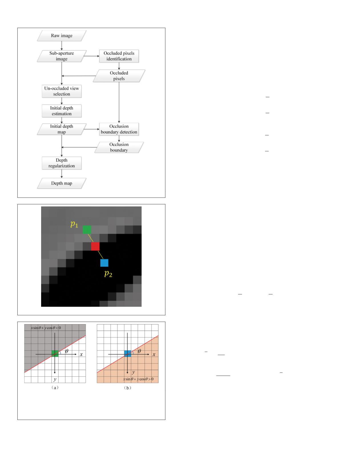
First, the orientation angle
θ
at each edge pixel is obtained
by applying the edge-orientation predictor on the edge. Then
two pixels on either side of the edge pixel are selected ac-
cording to Equations 1 and 2 as shown in Figure 8. Next, one
region of pixels in the angular patch of pixel
p
1
is selected ac-
cording to Equation 3 as shown in Figure 9a, and one region
of pixels in the angular patch of pixel
p
2
is selected according
to Equation 4 as shown in Figure 9b.
x
x
y
y
1
1
2
2
0 5
2
2
=
+
+
+
=
−
+
floor
floor
cos
.
sin
θ π
θ π
+
0 5.
(1)
x
x
y
y
2
2
2
2
0 5
2
2
=
−
+
+
=
+
+
floor
floor
cos
.
sin
θ π
θ π
+
0 5.
,
(2)
where (
x
1
,
y
1
) is the coordinates of pixel
p
1
in Fig. 8, (
x
,
y
) is
the coordinates of the edge pixel, and (
x
2
,
y
2
) is the coordi-
nates of pixel
p
2
.
x
sin
θ
+
y
cos
θ
< 0
(3)
x
sin
θ
+
y
cos
θ
> 0
(4)
If the edge pixel is not occluded, two pixels
p
1
and
p
2
on
either side of the edge pixel will be at the same or similar
depth; when the two regions of pixels in the angular patch re-
focus to the corresponding object point at the same or similar
depth, the variances of the two regions will be minimal. If the
edge pixel is occluded, when the pixels in one region refocus
to the correct depth, having the minimum variance, the pixels
in the other region still have large variance. Therefore, the re-
focused depth will be different when the two regions of pixels
minimize variance. According to this feature, the occluded
pixels can be identified from the edge pixels.
For the two pixels, we refocus to different depths using the
4D light field (Ng
et al.
2005):
L x y u v L x u
y v
u v j
j
j
α
α
α
,
, , ,
,
, , ,
,
(
)
= + −
+ −
=
1
1
1
1
1 2 , (5)
where
L
j
is the input light field,
α
is the ratio of the refocused
depth to the current focused depth,
L
α
,
j
is the refocused light
field, (
x
,
y
) is the spatial coordinates in the center-view image,
and (
u
,
v
) is the angular coordinates. The center view is located
at (
u
,
v
) = (0, 0). This provides an angular patch for each depth.
We first compute the means and variances of the two regions:
L
N
L x y u v j
j
j
j
j
j
u v
j
j
α
α
,
,
,
, , , ,
,
=
(
)
=
∑
1
1 2
(6)
,
,
(
)
V x y
N
L x y u v L x y
j
j
j
j
j
j
u v
j
j
α
α
α
,
,
,
,
, ,
,
(
)
=
−
(
)
−
(
)
∑
1
1
2
,
(7)
where
N
j
is the number of pixels in region
j
.
Then the optimal depth of the two regions is determined as
j
j
α
α
α
V x y
*
,
,
=
(
)
argmin
.
(8)
Figure 7. Flowchart of the proposed depth-estimation method.
Figure 8. The selection of adjacent pixels.
Figure 9. The selected pixels in angular patches of pixels
p
1
and
p
2
. (a) The gray pixels in the angular patch of pixel
p
1
are selected. (b) The orange pixels in the angular patch of
pixel
p
2
are selected. The line equation is determined by the
orientation angle
θ
of the edge pixel.
446
July 2020
PHOTOGRAMMETRIC ENGINEERING & REMOTE SENSING


