views. The cost volumes
C
(
x,y,l
) are defined by combining the
refocus
C
r
(
x,y,l
) and correspondence
C
c
(
x,y,l
) cues as
C x y l
C x y l
C x y l
, ,
, ,
, ,
(
)
=
(
)
+ −
(
)
(
)
α
α
r
c
1
(14)
where
α
∈
(0,1) adjusts the relative importance between the
defocus cost
C
r
and the correspondence cost
C
c
. Here,
α
is set
to 0.5. The cost volumes are computed based on the subpixel
shifts of subaperture images using the phase-shift theorem
(Jeon
et al.
2015):
I x x F F I x
i x
+
(
)
=
( )
{ }
{
}
−
∆
∆
1
2
exp
π
,
(15)
where
I
(
x
) is an image,
I
(
x
+
Δ
x
) is the subpixel image shifted
by
Δ
x
,
F
{·} denotes the discrete 2D Fourier transform, and
F
{·}
denotes the inverse discrete 2D Fourier transform. Therefore,
the defocus cue is defined as
I x y l
N
I x d y d
u v
u
v
u v
, ,
,
,
,
(
)
=
+ +
(
)
∑
1
(16)
C x y l
N
I x y l I x d y d
u v
u
v
u v
r
, ,
, ,
,
,
,
(
)
=
-
(
)
-
+ +
(
)
∑
1
1
2
, (17)
where
N
is the number of unoccluded views,
l
is the cost
label, (
u,v
) are unoccluded views,
I
u,v
denotes the images
corresponding to the unoccluded views, (
x,y
) is the spatial
coordinates, and the subpixel shifts
d
u
and
d
v
are defined as
d
d
kl u u
kl v v
u
v
=
-
(
)
-
(
)
c
c
,
(18)
where
k
is the unit of the label in pixels and (
u
c
,v
c
) is the
center view.
The correspondence cue is defined as
C x y l
I x y l I
x y
u v
c c
c
, ,
, ,
,
,
(
)
=
(
)
-
(
)
2
,
(19)
where
I
u
c
,
v
c
is the center-view image.
Then the initial depth map is obtained by minimizing the
cost volumes:
l x y
C x y l
l
d
argmin
,
, ,
(
)
=
(
)
.
(20)
Depth Regularization
In this section, the occlusion boundary is detected and the
initial depth map is refined with global regularization using
an energy function.
Occlusion-Boundary Detection
We find the occlusion boundary by combining the depth cues
and the occluded pixels obtained previously.
For an occluded pixel in an occlusion boundary, the depth
gradient is larger than for an unoccluded pixel. So we can get
an initial occlusion boundary by computing and thresholding
the gradient of the initial depth:
Occ_d
if
if
d
d
d
d
=
∇
>
∇
≤
1
0
N
N
l
l
l
l
ε
ε
,
(21)
where
l
d
is the initial depth and
Δ
l
d
is the gradient of the
initial depth. Since the depth gradient becomes larger as the
depth becomes greater, we divide the gradient
Δ
l
d
by
l
d
to
increase robustness.
N
(·) is a normalization function that sub-
tracts the mean and divides by the standard deviation. Here
the threshold
ε
is set to 1.
The occlusion boundary can be computed by
Occ Occ_d Occ_c
=
∩
,
(22)
where Occ_c is the occluded pixels obtained previously. An
example is shown in Figure 16.
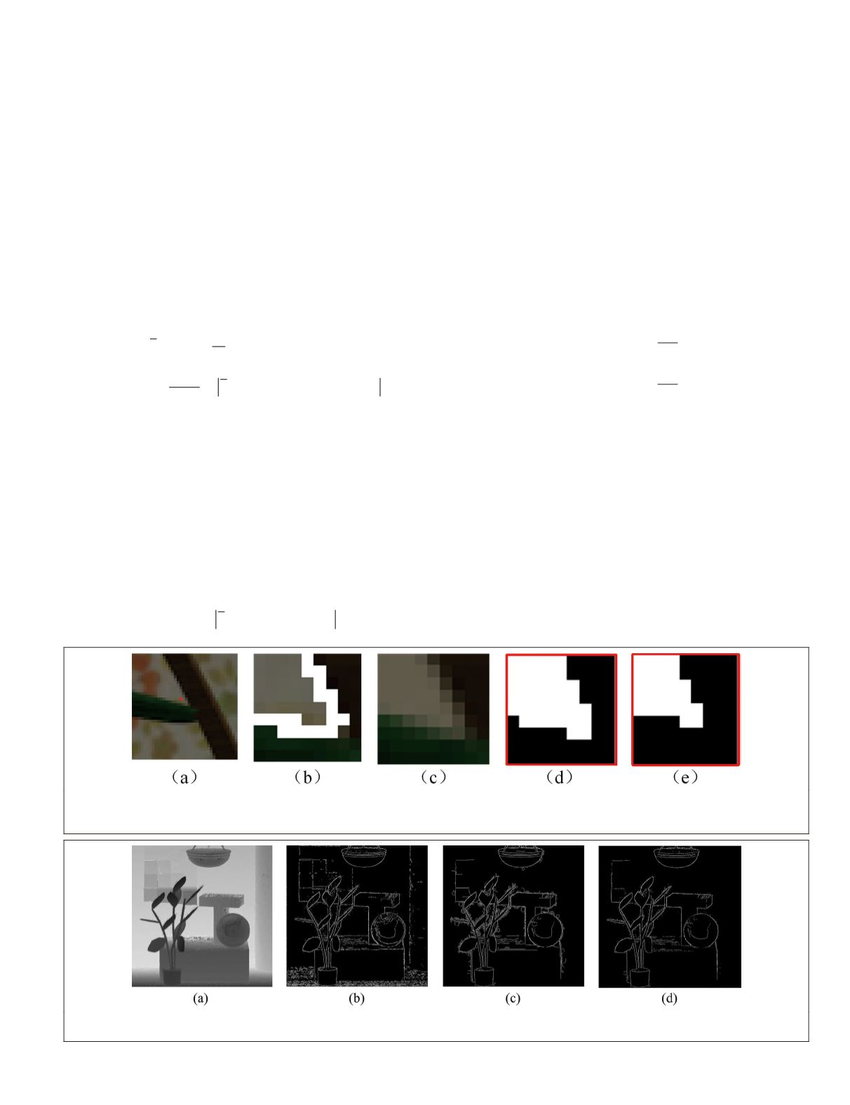
Figure 15. Refined unoccluded views. (a) The close-up image in the Mona data set. (b) The spatial patch corresponding to the
red point in (a); white pixels are the edge pixels. (c) The angular patch, when refocused to the correct depth, of the red point
in (a). (d) Our selected unoccluded views. (e) The refined unoccluded views after removal of the edge pixels.
Figure 16. The detected occlusion boundary. (a) The initial depth map of the Mona data set. (b) The initial occlusion
boundary Occ_d. (c) The occlusion pixels obtained using our method. (d) The occlusion boundary Occ.
PHOTOGRAMMETRIC ENGINEERING & REMOTE SENSING
July 2020
449


