combine region 1 with the other two categories to get another
two regions, marked as region 2 and region 3, respectively.
Then the angular patch is divided into the same regions as the
spatial patch and an adaptive strategy is used to obtain the
optimal unoccluded views. First, we compute the means
L
α
,j
and variances
V
α
,j
of the three regions using Equations 6 and
7. Then, we find the depth
α
*
j
corresponding to the minimum
of the three regions using Equation 8. The minimum variance
and mean corresponding to the depth
α
*
j
are
V V x y
j
j
j
min,
,
*
,
=
(
)
α
(10)
L L
j
j
j
=
α
*
,
.
(11)
Let
j
V
j
j
*
,
=
argmin
min
(12)
be the index of the region that exhibits minimum variance.
If
j
*
= 2 or 3, the region
j
*
in the angular patch is the optimal
unoccluded views. If
j
*
= 1, the index
j
u
of the region cor-
responding to the optimal unoccluded views is selected by
comparing the means of the three regions:
j
L L
j j
L L
L L
j
u
if
if
if
=
- >
≠
- <
- <
1
2
3
1
1
2 1
3 1
,
:
,
(13)
where
ϵ
is a threshold value which is set to 0.01. Now the un-
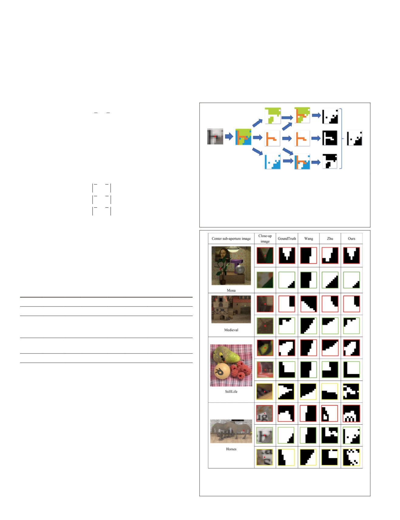
occluded views of the occluded pixel are shown in Figure 13.
In order to verify the effectiveness of the proposed method
to select unoccluded views, the F-measure (Sasaki 2007) of
the unoccluded views in occlusion using our algorithm is
computed and compared with previous work (T.-C. Wang
et
al.
2016; Zhu
et al.
2017). The quantitative comparisons are
listed in Table 1. The qualitative comparisons of the unoc-
cluded views are shown in Figure 14.
Table 1. F-measures for unoccluded-view selection.
Data Set
Method Buddha Mona Medieval Horse StillLife Papillon Average
T.-C.
Wang
et
al.
(2016)
0.61 0.65 0.52 0.56 0.54 0.59 0.58
Zhu
et
al.
(2017)
0.70 0.75 0.61 0.61 0.68 0.71 0.68
Ours
0.78 0.83 0.80 0.80 0.78 0.79 0.80
As can be seen from Table 1 and Figure 14, our algorithm
can select more accurate unoccluded views and has more
obvious advantages in the multi-occluder areas. The unoc-
cluded views selected in the method of T.-C. Wang
et al.
(2016) always include some occluded views, resulting in
oversmoothness in the multi-occluded areas. The method of
Zhu
et al.
(2017) selects more accurate unoccluded views,
but its accuracy is lower than that of our algorithm. In the
StillLife data set, the red point in the yellow box is occluded
by two objects. The selection of unoccluded views in the
methods of T.-C. Wang
et al.
and Zhu
et al.
fail, while our
algorithm still selects the most accurate unoccluded views. In
the Horses data set, there are many textures near the occluded
points in the background (the red, green, and yellow boxes),
and the methods of T.-C. Wang
et al.
and Zhu et al select some
occluded views. Although our method does not select all
the unoccluded views, the selected views are all unoccluded
views, which can avoid oversmoothing.
In order to eliminate the aliasing influence of edge pixels
in the angular patch, selected unoccluded views correspond-
ing to the edge pixels in the spatial patch are removed, as
shown in Figure 15. Consequently, the accuracy of depth esti-
mation can be improved using the refined unoccluded views.
Initial Depth Estimation
After selection of the unoccluded views, the initial depth map
is obtained by computing the cost volumes in the unoccluded
Figure 13. Selection of unoccluded views (three categories).
The first two columns represent that the spatial patch of one
occluded pixel is divided into three categories by affinity
propagation. The third and fourth columns represent that
the spatial patch is divided into three regions. The fourth
and fifth columns represent that the angular patch is
divided into the same regions (white) as the spatial patch.
The last column represents the selected unoccluded views.
Figure 14. Comparisons of unoccluded-view selection.
White areas denote the selected unoccluded views. All the
data sets are from Wanner
et al.
(2013).
448
July 2020
PHOTOGRAMMETRIC ENGINEERING & REMOTE SENSING


