The error matrices of three indices were also tested to de-
termine if they differed significantly and to determine which
was most accurate. The Z-statistic for testing pairs of error
matrices was calculated as:
Z
–
=
(
)
+
(
)
KHAT KHAT
var KHAT var KHAT
1
2
1
2
where KHAT
1
and KHAT
2
are estimates of the Kappa statistic
and var(KHAT
1
) and var(KHAT
2
) are estimates of the variance
for index #1 and index #2, respectively (Congalton and Green,
2008). We compared FCI1 to FCI2, FCI1 to
NDVI
, and FCI2 to
NDVI
and used Z
≥
1.96 (p
≤
0.05) to determine which ones
were significantly different.
Results
Overview of Spectral Distinctions Between Trees and Other Land Covers
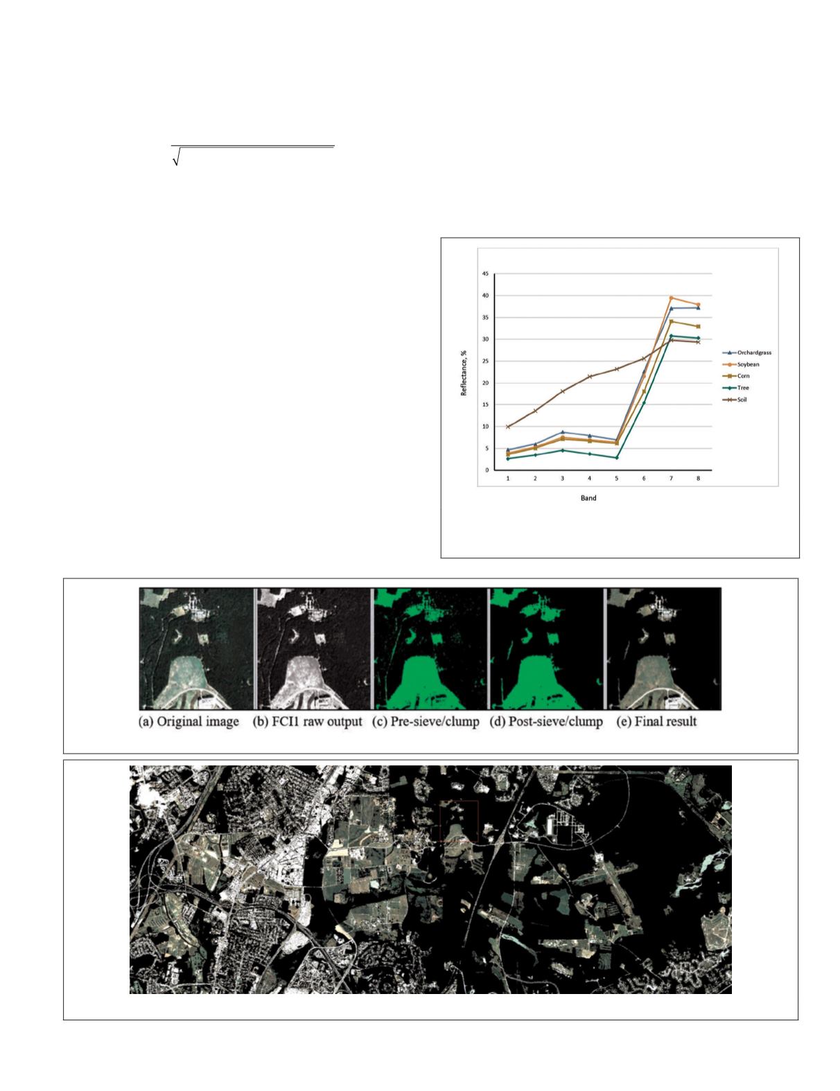
All healthy green vegetation follows roughly the same shaped
spectral curve with variations based on factors such as health,
water content, and structure of the mesophyll layer (Figure
2; Knipling, 1970). In Figure 2, green vegetation has low
reflectance in the visible (400 to 700 nm) portion in the elec-
tromagnetic spectrum, before increasing sharply into the near
infrared (700 to 1,100 nm) portion making it distinct from
other land covers (Dozier, 1989; Huete and Jackson, 1987; and
Nagler
et al
., 2000). The red edge band (Table 1) captures the
transition between the red and near infrared (
NIR
) bands and
provides additional information about plant chlorophyll sta-
tus (Horler
et al
., 1983), which may help distinguish between
vegetation covers. Pu and Landry (2012) used WordView-2
to map urban tree species and found that the presence of the
red edge band improved the results. Heenkenda
et al.
(2014)
substituted the red edge for the red band in the Normalized
Difference Vegetation Index (
NDVI
) and differentiated between
home gardens and other vegetation. These variations are
unique enough to discriminate forest cover from other vegeta-
tion types and can be exploited with the development of a
spectral index.
Forest Cover Index Output
The workflow to apply the FCI1 and FCI2 to imagery yielded
raster images in which pixels containing trees were success-
fully masked while pixels containing other vegetative land
covers remained visible (Figures 3 and 4). Tree pixels were
among the darkest pixels in the imagery with the majority of
Figure 3. (a to e) This figure illustrates the steps in each part of the FCI workflow in a 05 August 2012 image.
Figure 4. This figure shows the result of the FCI1. Forest cover is masked out of the image.
Figure 2. WorldView-2 spectral profiles of land covers taken
from an average of multiple pixels in the study area from 05
August 2012 imagery.
PHOTOGRAMMETRIC ENGINEERING & REMOTE SENSING
August 2018
509


